Using the Smith Chart to Design a T and Pi Matching Network

Impedance matching networks are a core part of an RF circuit. By transforming the load impedance to a desired value, we can ensure that certain performance conditions, such as maximum power transfer, are met.

In the previous article, we saw that two-element lumped networks, known as L-sections, can be used to provide impedance matching at a certain frequency. While L-sections are widely used, they don’t give us the flexibility to choose the bandwidth. The bandwidth of these circuits is constant for a given input and output impedance. With that in mind, there are often many applications where we need to have control over the bandwidth of the matching network. When a narrower bandwidth than that of an L-section is required, more complicated arrangements, such as T or Pi networks, should be employed.

This article delves into a discussion on the design of these types of matching networks using a Smith chart. The Smith chart was an invention of the electrical engineer Phillip Hagar Smith.

 

Smith Chart Constant-Q Circles

Before diving in too far, it’s important to familiarize ourselves with constant-Q circles on a Smith chart. Previously, we defined the nodal Q of a circuit node with impedance Z = R + jX as:

 

\[Q_n=\frac{|X|}{R}\]

 

We also discussed that the maximum Q_n specifies the quality factor—and thus the bandwidth—of an L-section. With Smith charts, we prefer to use the normalized impedances z = r + jx. Even with normalized impedances, we can still use the above equation because both the numerator and denominator are divided by the same normalizing factor. Therefore, we attain Equation 1: 

 

\[Q_n=\frac{|x|}{r}\]

Equation 1.

 

There are an infinite number of points on the Smith chart that produce the same Q_n. For example, points z₁ = 0.2 + j0.2, z₂ = 0.5 + j0.5, z₃ = 1 + j, and z₄ = 2 + j2 all correspond to Q_n = 1. The constant-Q curve of Q_n = 1 is shown in the following Smith chart in Figure 1.

 

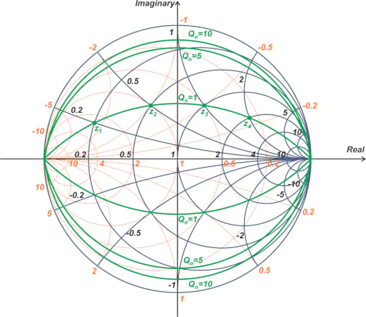
Figure 1. Smith chart showing the constant-Q curve of Q_n = 1.

 

According to Equation 1, the complex conjugate of z₁, z₂, z_3, and z₄ also produces Q_n = 1. These points also correspond to another Q_n = 1 curve at the lower half of the Smith chart. Additionally, the above figure shows constant-Q contours of Q_n = 5 and 10. It can be shown that impedances with Q_n = a transform into two circles in the Γ-plane. Both circles are of radius \(\sqrt{1+\frac{1}{a^2}}\), one centered at (0, -1/a) and the other centered at (0, 1/a). For more information on this, I suggest reading the book "Microwave Transistor Amplifiers: Analysis and Design" by Guillermo Gonzalez.

 

T-type Matching Networks: The Basic Idea

We’ll explain this method through an example. Consider transforming z_Load = 0.2 to the center of the Smith chart. One option for this impedance transformation is to use a two-element matching network corresponding to the cyan path shown below (Figure 2). 

 

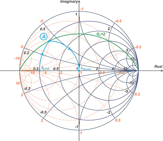
Figure 2. Smith chart showing the impedance transform using a two-element matching network corresponding to the cyan path (A).

 

Since only two motions are allowed to go from z_Load to z_Source, the intermediate impedance has to be at the intersection of the r = 0.2 and g = 1 circle (point A in the figure). This means that, with a two-element network, we cannot adjust the location of the intermediate impedance, and thus, the quality factor of the circuit is fixed. As we can see, the intersection point lies on the Q_n = 2 circle in our example. You might wonder what happens if we continue our motion along the r = 0.2 circle to some point above point A. This is shown in Figure 3.

 

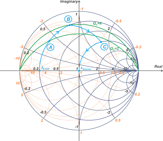
Figure 3. Smith chart showing the r = 0.2 circle.

 

In the above example, we move to point B rather than point A, producing a Q_n of 4. However, we now need at least two additional motions to go from point B to the center of the chart. The first motion is along the g = 0.3 constant-conductance circle, and the second motion is along the r = 1 constant-resistance circle. The path shown in the above figure needs two series components and one parallel component, leading to a T-type matching network, as shown in Figure 4.

 

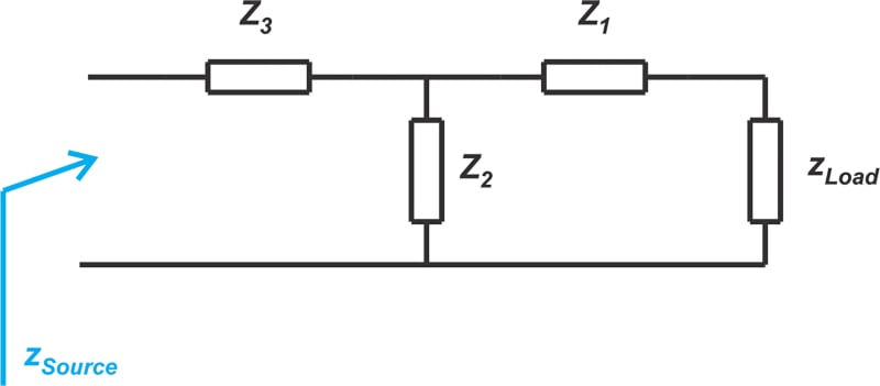
Figure 4. Creating a T-type matching network using two series and one parallel component.

 

The above circuit allows us to increase the maximum nodal Q from 2 to 4, however, at the cost of using a three-element matching network. Referring to a more complete Smith chart, we can now find the reactance and susceptance of the intermediate points A, B, and C for the above impedance matching solutions. This information is provided in Table 1.

 

Table 1. The reactance and susceptance for points A, B, and C.

Intermediate Point	Reactance (x)	Susceptance (b)
A	0.4	-2
B	0.8	-1.2
C	1.53	-0.47

 

Let’s find the component values and compare the frequency response of these two circuits.

 

Finding Component Values, Responses, and Bandwidth

Below we'll show you how to find the component values for an L-section and a T-network, as well as the frequency response and bandwidth of these matching network techniques.

 

Finding L-section Component Values

Assume that the normalizing impedance is Z₀ = 50 Ω, and the frequency of interest is 1 GHz. The component values of the L-section can be found as follows. The motion from z_Load to point A corresponds to a series inductor with a normalized reactance of x_A - x_Load = j0.4 - j0 = j0.4. This requires a 3.18 nH series inductor at 1 GHz.

The motion from point A to z_Source in Figure 2 requires a parallel capacitor with a susceptance of b_Source - b_A = 0j - (-j2) = j2. This can be produced by a 6.37 pF parallel capacitor. The final L-section is shown in Figure 5.

 

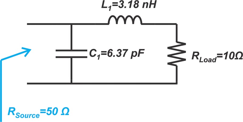
Figure 5. Example L-section diagram.

 

Finding T-network Component Values

Next, we can find the component values of the T-network in a similar manner. In this case, the motion from z_Load to point B corresponds to a series inductor with the normalized reactance of j0.8 that can be produced by a 6.37 nH inductor. The next motion requires a capacitive susceptance of b_C - b_B = -j0.47 - (-j1.2) = j0.73 that can be obtained by a 2.32 pF capacitor. Finally, we need a series capacitor with reactance -j1.53 to go to the center of the chart, which can be achieved by a 2.08 pF capacitor. The final T-network is shown in Figure 6.

 

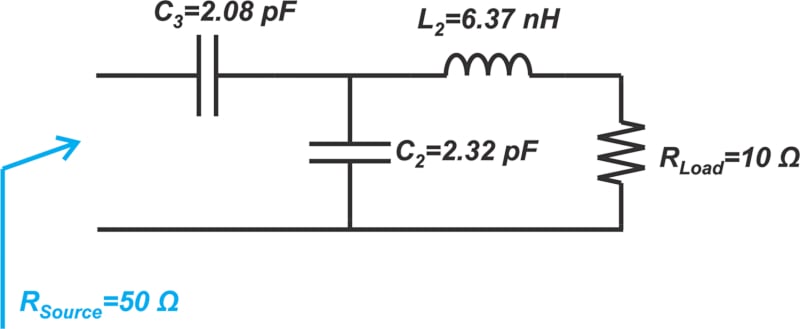
Figure 6. Example T-network diagram.

 

L-section and T-network Frequency Response and Bandwidth

The frequency response of these two circuits is shown in Figure 7.

 

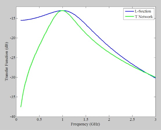
Figure 7. T-network and L-section frequency responses. 

 

The L-section has a lowpass response with an upper 3 dB cut-off of 1.46 GHz. Below 1 GHz, the circuit doesn’t have a 3 dB cut-off frequency. This is due to the low Q of the circuit. If we assume that the response is symmetric around 1 GHz, we can approximate the bandwidth as 21.46-1=0.92 GHz.

Let’s use our knowledge from the previous article to verify this value. We know that the quality factor Q_L of an L-section is one-half its maximum nodal Q (Q_n). From Figure 2, we have Q_n = 2 and thus Q_L = 1. Therefore, the bandwidth should be:

 

\[BW=\frac{f_0}{Q_L}=\frac{1 \text{ } GHZ}{1}=1 \text{ }GHz\]

 

This equation is in reasonable agreement with the simulation result. On the other hand, for the T-network, the upper and lower 3 dB points are at 1.29 GHz and 750 MHz, leading to a bandwidth of 540 MHz. As we can see, a T-network allows us to increase the nodal Q of the circuit and achieve a lower bandwidth than that of an L-section. It is not simple to exactly relate Q_n to Q_L in a T-network (this is also true for Pi networks, which we’ll get into shortly). However, the Q of a T or Pi network is normally taken as the highest value of Q_n in the circuit.

 

Can We Reduce Q_n Through a T Network?

The above discussion shows that a T-network can produce a Q_n larger than that of an L-section. The question that arises now is, can we use a T-network to reduce Q_n to below that of an L-section? To answer this question, consider the Smith chart in Figure 8.

 

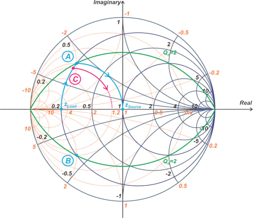
Figure 8. Smith chart with an intermediate impedance at point C.

 

In the above figure, we have chosen the intermediate impedance at point C that has a Q_n lower than 2. Since we aim to have a T-network, we should continue our motion along the constant-conductance circle passing through point C (the g = 1.2 circle in our example). To have a three-element network, the g = 1.2 circle must intersect the r = 1 circle that goes through z_Source. However, the above diagram shows that if the intermediate point C has a Q_n less than 2, the constant-conductance circle going through C doesn’t intersect the r = 1 circle. Therefore, it is not possible to have a T-network with Q_n less than that of the L-section.

 

Designing a Pi Matching Network

Another type of three-element matching network is the Pi network depicted below (Figure 9).

 

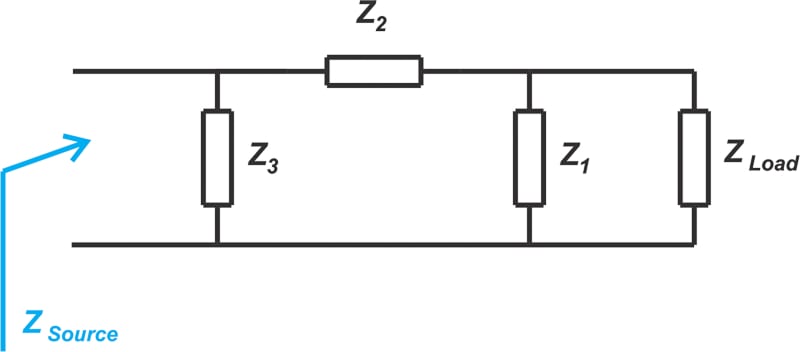
Figure 9. Pi network diagram example.

 

Let’s design a Pi network to transform z_Load = 3.33 to the center of the Smith chart at 1 GHz. Assume that the maximum Q_n is asked to be 4. With a Pi circuit, the elements next to Z_Load and Z_Source are parallel components, and thus, we’re allowed to move along constant-conductance circles going through the source and load impedances. An intersection of these constant-conductance circles and the Q_n = 4 curve can be used as an intermediate point, as shown in Figure 10.

 

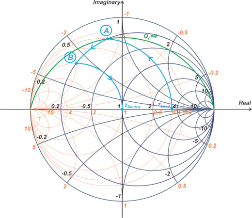
Figure 10. Smith chart showing constant-conductance circles and a Q_n = 4 curve as an intermediate point.

 

In this example, the g = 0.3 circle is the constant-conductance circle that goes through z_Load. The intersection of this circle with the Q_n = 4 curve (point A above) is used as the intermediate point for impedance transformation. The next move should be along the constant-resistance circle going through point A (this corresponds to the series component of the Pi network). In our example, the r = 0.2 circle is the constant-resistance circle that goes through point A. The intersection of the r = 0.2 circle and the g = 1 constant-conductance circle is our next intermediate impedance (point B). Finally, we move along the g = 1 circle to reach the center of the Smith chart. Using a more complete Smith chart, we can find the reactance (x) and susceptance (b) of points A and B, as provided in Table 2.

 

Table 2. The reactance and susceptance for points A and B.

Intermediate Point	Reactance (x)	Susceptance (b)
A	0.8	-1.2
B	0.4	-2

 

Using this information, we can find the component values. The motion from z_Load to point A requires a normalized susceptance of -j1.2 that can be achieved by a 6.63 nH parallel inductor at 1 GHz (assuming Z₀ = 50 Ω). The motion from point A to B requires a normalized reactance of j0.4 - j0.8 = -j0.4 that can be obtained by a 7.96 pF series capacitor. Finally, the motion from B to z_Source needs a normalized susceptance of j2 that leads to a 6.37 pF parallel capacitor. The final circuit is shown in Figure 11.

 

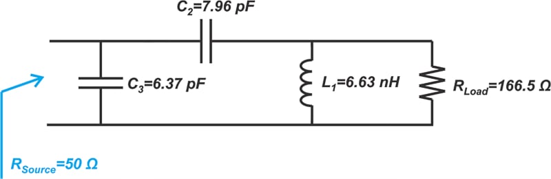
Figure 11. Pi network schematic.

 

The frequency response of the circuit is shown below.

 

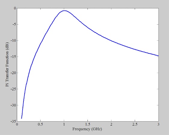
Figure 12. Pi network frequency response.

 

For the Pi network, the upper and lower 3dB points are at 1.3 GHz and 780 MHz, leading to a bandwidth of about 520 MHz.

 

Using T and Pi Matching Networks Summary

While L-sections are quite practical circuits, they don’t give us the flexibility to choose the bandwidth. The bandwidth of these circuits is constant for a given input and output impedance. When a narrower bandwidth than that of an L-section is required, more complicated arrangements, such as T or Pi networks, can be employed. Keep in mind that these types of networks can only increase the quality factor (or equivalently reduce the bandwidth) of the circuit. In the next article, we’ll look at matching circuits that can provide a wider bandwidth than a simple L-section.

 

---

 

To see a complete list of my articles, please visit this page.