Use Signal Averaging to Increase the Accuracy of Your Measurements
In this article, we'll discuss the signal averaging method, a noise reduction technique, and how it can help increase the accuracy of your signal measurements.
Our measurements are inevitably affected by the noise that can come from different sources. Sometimes the signal that we measure is orders of magnitude smaller than the noise component. In these cases, we need noise reduction techniques to somehow suppress the noise. In this article, we’ll look at the signal averaging method that, in particular cases, can be very effective.
How Does Signal Averaging Work?
Assume that the output of an experiment is an exponential curve as shown in Figure 1.
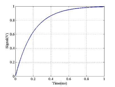
Figure 1
Suppose that our measurement setup uses an ADC to digitize this signal. We ideally expect to have the samples of the curve in Figure 1; however, in reality, a noise voltage appears at the ADC input and corrupts our samples. Assume that the noise component has a normal distribution with a mean value of 0 and a variance of 1. An example of such a noise component is shown in Figure 2.
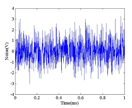
Figure 2
If we add the above noise component to the desired output shown in Figure 1, we obtain the waveform in Figure 3.
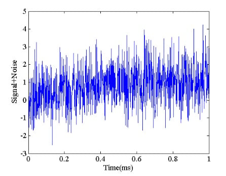
Figure 3
As you can see, the noise is large enough to bury the desired output. How can we achieve a more accurate measurement? Actually, this is theoretically possible if certain assumptions are valid about the noise component. Let’s assume that the noise samples are neither correlated with each other nor the desired output. Also, suppose that the mean value of the noise is zero. Now, let’s repeat this experiment three times as shown in Figure 4.
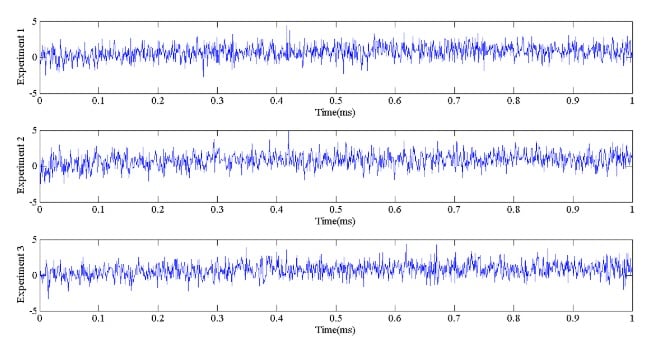
Figure 4
At t=0.3 ms, we have the following values from these three experiments:
X1 = S1 + n1 = -0.707 v
X2 = S2 + n2 = 1.712 v
X3 = S3 + n3 = 2.557 v
In the above equations, Si for i = 1, 2, 3 denotes the desired signal value which is 0.7769 v in this particular example (from Figure 1). However, ni which is the noise component, varies from one experiment to the other. Since the noise samples are not correlated with each other and have a zero mean, averaging the above three values should give a better estimate of the desired value. We obtain:
Xaverage = 1.187 v
Note that the desired value, which is the same in all of our experiments, is not suppressed by the averaging process; however, the noise component that is random and has a zero mean becomes smaller. Figure 5 shows the signal that we get by calculating the average of the three experiments. Although the average is still very noisy, its overall shape somehow resembles the exponential curve in Figure 1.
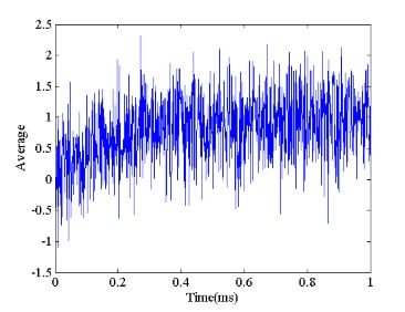
Figure 5
Is it possible to improve the accuracy by increasing the number of experiments? Figure 6 shows the averaged output for 100, 200, 300, and 400 experiments.
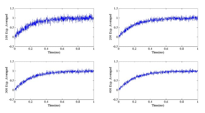
Figure 6
As we increase the number of experiments, we get a more and more accurate measurement. Let’s take a look at the mathematical analysis of the averaging and quantify the effect of increasing the number of experiments on the noise suppression.
Mathematical Analysis
Assume that an experiment can be repeated over N trials. If we denote the experiment number with j, the output of the j-th experiment, Xj, can be written as
Xj = S + nj 1 ≤ j ≤ N
where S denotes the desired output which is the same for all of these N trials, and nj is the noise component affecting the j-th experiment. Unlike the desired output, the noise component varies from one experiment to the other. Suppose that, to digitize our measurements, we take a total of M samples from the output of each experiment. If we represent the sample number with k, we have
Xj(k) = S(k) + nj(k) 1 ≤ k ≤ M
Therefore, for a given sample number p, we have N different values from these experiments:
X1(p) = S(p) + n1(p)
X2(p) = S(p) + n2(p)
…
XM(p) = S(p) + nM(p)
We saw that signal averaging can suppress the noise component. The average of these values is
\[X_{Avg}(p)=\frac {1}{M} \sum_{j=1}^{M} \left ( S(p)+n_j(p) \right )\]
Since S(p) is the same for all of these experiments, we have
\[X_{Avg}(p)=S(p) + \frac {1}{M} \sum_{j=1}^{M} n_j(p) =S(p)+n(p)\]
We don’t know the exact value of the noise sample nj(p) that is affecting the j-th experiment but we assume that it is a random variable with zero mean and variance σn2. To quantify the effect of signal averaging on noise reduction, we should calculate the variance of the averaged noise component n(p) that we will denote by σn, avg2. We know that variance can be found by the following equation:
\[{\sigma _{n, avg} }^2 =E\left ([n(p)]^2 \right ) - \mu^2\]
where E(.) denotes the expected value and μ is the mean value of n(p). Since the random variables nj(p) are assumed to have a zero mean, the mean value of n(p) will be zero as well. Hence, we have
\[{\sigma _{n, avg} }^2 =E\left ([n(p)]^2 \right ) =E\left [ \frac{1}{M}\sum_{j=1}^M n_j(p)\right ]^2 = E\left ( \frac{1}{M^2}\sum_{j=1}^M n_j(p) \sum_{j=1}^M n_j(p) \right )\]
This can be rewritten as
\[{\sigma _{n, avg} }^2 = E\left ( \frac{1}{M^2}\sum_{j=1}^M \sum_{j=1}^M n_j(p) n_j(p) \right ) = \frac{1}{M^2}\sum_{j=1}^M \sum_{j=1}^M E\left ( n_j(p) n_j(p) \right )\]
If you need to review the properties of the expectation operator, please see this video. The above summation has a total of M2 terms. Some of them involve multiplying two different random variables, i.e. ni(p)nj(p) where i≠j. For these terms, since we assumed that the random variables are independent, we have:
\[E(n_i(p)n_j(p))=E(n_i(p))E(n_j(p))=0 \; \; \; \; for \; \; \; i \neq j\]
because the expected value of each of these random variables is zero. However, for the terms that i=j, we obtain
\[E\left ( n_i(p)n_j(p) \right )=E\left ( \left [ n_i(p) \right ]^2 \right )= {\sigma_n}^2 \; \; \; \; for \; \; \; i = j\]
There are a total of M such terms, hence we obtain:
\[{\sigma _{n, avg} }^2 = \frac{1}{M^2}\sum_{j=1}^M \sum_{j=1}^M E \left( n_j(p) n_j(p) \right ) = \frac{1}{M^2}M {\sigma_n}^2 = \frac{{\sigma_n}^2}{M}\]
The above equation shows that while the variance of noise samples was σn2, the signal averaging technique reduces it by a factor of M. Note that the desired signal is not affected by the averaging. Hence, we can conclude that signal averaging can increase the signal to noise ratio (SNR) by a factor of M. This analysis allows us to choose the desired number of experiments for the averaging technique so that we can achieve an arbitrary SNR.
By understanding the above analysis, we can have better insight into the limitations of the signal averaging technique. The implied assumptions for the above analysis are:
- The noise can be modeled by a random variable with zero mean
- Signal and noise are not correlated
- The noise samples are not correlated with each other
- The experiment is repeatable
Signal Averaging Relies on the Noise Randomness
Sometimes the noise that appears at the input of our measurement system is not really random. For example, the noise coming from the power line can create a non-random noise component. Assume that the power line frequency is 50 Hz (a period of 20 ms) and we trigger our measurements every 40 ms. This is shown in Figure 7. In this case, the noise that affects a particular sample, n(k), is always related to a particular part of the power line sinusoid. Hence, the averaging technique will not suppress this noise. To resolve this issue, we can simply choose a measurement cycle that is not divisible by 20 ms. Alternatively, we can use a randomized measurement cycle.
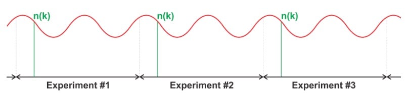
Figure 7
Conclusion
Sometimes the signal that we measure is orders of magnitude smaller than the noise component. In these cases, we need noise reduction techniques to somehow suppress the noise. In this article, we looked at the signal averaging technique that can be helpful when the noise is not correlated with our desired signal. Moreover, the noise should have a zero mean. We saw that if we repeat an experiment M times and calculate the average of these experiments, the signal to noise ratio (SNR) can be improved by a factor of M.
To see a complete list of my articles, please visit this page.