Understanding Training Formulas and Backpropagation for Multilayer Perceptrons

Welcome to AAC's series on machine learning.

Catch up on the series so far here:

1. How to Perform Classification Using a Neural Network: What Is the Perceptron?
2. How to Use a Simple Perceptron Neural Network Example to Classify Data
3. How to Train a Basic Perceptron Neural Network
4. Understanding Simple Neural Network Training
5. An Introduction to Training Theory for Neural Networks
6. Understanding Learning Rate in Neural Networks
7. Advanced Machine Learning with the Multilayer Perceptron
8. The Sigmoid Activation Function: Activation in Multilayer Perceptron Neural Networks
9. How to Train a Multilayer Perceptron Neural Network
10. Understanding Training Formulas and Backpropagation for Multilayer Perceptrons
11. Neural Network Architecture for a Python Implementation
12. How to Create a Multilayer Perceptron Neural Network in Python
13. Signal Processing Using Neural Networks: Validation in Neural Network Design
14. Training Datasets for Neural Networks: How to Train and Validate a Python Neural Network

We’ve reached the point at which we need to carefully consider a fundamental topic within neural-network theory: the computational procedure that allows us to fine-tune the weights of a multilayer Perceptron (MLP) so that it can accurately classify input samples. This will lead us to the concept of “backpropagation,” which is an essential aspect of neural-network design.

Updating Weights

The information surrounding training for MLPs is complicated. To make matters worse, online resources use different terminology and symbols, and they even seem to come up with different results. However, I’m not sure if the results are truly different or just presenting the same information in different ways.

The equations contained in this article are based on the derivations and explanations provided by Dr. Dustin Stansbury in this blog post. His treatment is the best that I found, and it’s a great place to start if you want to delve into the mathematical and conceptual details of gradient descent and backpropagation.

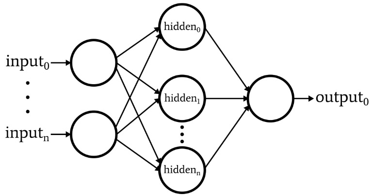
The following diagram represents the architecture that we’ll implement in software, and the equations below correspond to this architecture, which is discussed more thoroughly in the next article.

Terminology

This topic quickly becomes unmanageable if we don’t maintain clear terminology. I’ll be using the following terms:

• Preactivation (abbreviated \(S_{preA}\)): This refers to the signal (actually just a number within the context of one training iteration) that serves as the input to a node’s activation function. It is calculated by performing a dot product of an array containing weights and an array containing the values originating from nodes in the preceding layer. The dot product is equivalent to performing an element-wise multiplication of the two arrays and then summing the elements in the array resulting from that multiplication.
• Postactiviation (abbreviated \(S_{postA}\)): This refers to the signal (again, just a number within the context of an individual iteration) that exits a node. It is produced by applying the activation function to the preactivation signal. My preferred term for the activation function, denoted by \(f_{A}()\), is logistic rather than sigmoid.
• In the Python code, you will see weight matrices labeled with ItoH and HtoO. I use these identifiers because it is ambiguous to say something like “hidden-layer weights”—would these be the weights that are applied before the hidden layer or after the hidden layer? In my scheme, ItoH specifies the weights that are applied to values transferred from the input nodes to the hidden nodes, and HtoO specifies weights that are applied to values transferred from the hidden nodes to the output node.
• The correct output value for a training sample is referred to as the target and is denoted by T.
• Learning rate is abbreviated as LR.
• Final error is the difference between the postactivation signal from the output node (\(S_{postA,O}\)) and the target, calculated as \(FE = S_{postA,O} - T\).
• Error signal (\(S_{ERROR}\)) is the final error propagated back toward the hidden layer through the activation function of the output node.
• Gradient represents the contribution of a given weight to the error signal. We modify the weights by subtracting this contribution (multiplied by the learning rate if necessary).

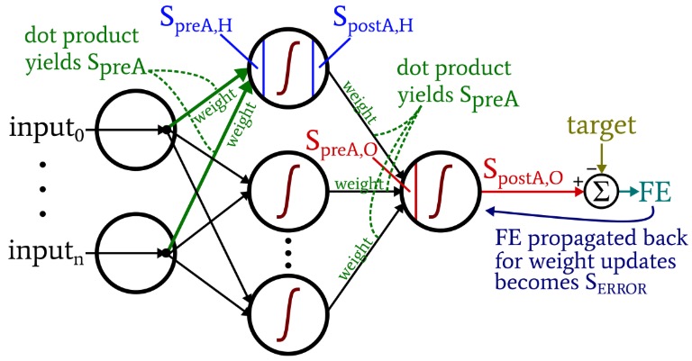
The following diagram situates some of these terms within the visualized configuration of the network. I know—it looks like a multicolored mess. I apologize. It’s an information-dense diagram, and though it may be a bit offensive at first glance, if you study it carefully I think that you will find it very helpful.

The weight-update equations are derived by taking the partial derivative of the error function (we’re using summed squared error, see Part 8 of the series, which deals with activation functions) with respect to the weight to be modified. Please refer to Dr. Stansbury’s post if you want to see the math; in this article we’ll skip straight to the results. For the hidden-to-output weights, we have the following:

\[S_{ERROR} = FE \times {f_A}'(S_{preA,O})\]

\[gradient_{HtoO}= S_{ERROR}\times S_{postA,H}\]

\[weight_{HtoO} = weight_{HtoO}- (LR \times gradient_{HtoO})\]

We calculate the error signal by multiplying the final error by the value that is produced when we apply the derivative of the activation function to the preactivation signal delivered to the output node (note the prime symbol, which indicates the first derivative, in \({f_A}'(S_{preA,O})\)). The gradient is then calculated by multiplying the error signal by the postactivation signal from the hidden layer. Finally, we update the weight by subtracting this gradient from the current weight value, and we can multiply the gradient by the learning rate if we want to change the step size.  

For the input-to-hidden weights, we have this:

\[gradient_{ItoH} = FE \times {f_A}'(S_{preA,O})\times weight_{HtoO} \times {f_A}'(S_{preA,H}) \times input\]

\[\Rightarrow gradient_{ItoH} = S_{ERROR} \times weight_{HtoO} \times {f_A}'(S_{preA,H})\times input\]

\[weight_{ItoH} = weight_{ItoH} - (LR \times gradient_{ItoH})\]
 

With the input-to-hidden weights, the error must be propagated back through an additional layer, and we do that by multiplying the error signal by the hidden-to-output weight connected to the hidden node of interest. Thus, if we’re updating an input-to-hidden weight that leads to the first hidden node, we multiply the error signal by the weight that connects the first hidden node to the output node. We then complete the calculation by performing multiplications analogous to those of the hidden-to-output weight updates: we apply the derivative of the activation function to the hidden node’s preactivation signal, and the “input” value can be thought of as the postactivation signal from the input node.

Backpropagation

The explanation above has already touched on the concept of backpropagation. I just want to briefly reinforce this concept and also ensure that you have explicit familiarity with this term, which appears frequently in discussions of neural networks.

Backpropagation allows us to overcome the hidden-node dilemma discussed in Part 8. We need to update the input-to-hidden weights based on the difference between the network’s generated output and the target output values supplied by the training data, but these weights influence the generated output indirectly.

Backpropagation refers to the technique whereby we send an error signal back toward one or more hidden layers and scale that error signal using both the weights emerging from a hidden node and the derivative of the hidden node’s activation function. The overall procedure serves as a way of updating a weight based on the weight’s contribution to the output error, even though that contribution is obscured by the indirect relationship between an input-to-hidden weight and the generated output value.

Conclusion

We’ve covered a lot of important material. I think that we have some really valuable information about neural-network training in this article, and I hope that you agree. The series is going to start getting even more exciting, so check back for new installments.