The Nyquist–Shannon Theorem in the Frequency Domain

In the previous article introducing the Nyquist-Shannon theorem, we saw that the frequency characteristics of a sinusoid are irretrievably lost when the waveform is sampled at a frequency that does not provide at least two samples per cycle. In other words, we cannot perfectly reconstruct the sinusoid if we sample at a frequency that is lower than the Nyquist rate.

Most signals, however, are not single-frequency sinusoids. For example, a modulated RF signal has frequencies associated with the carrier and the baseband waveform, and an audio signal representing human speech will cover a range of frequencies. 

We use the Fourier transform to visualize the frequency content of a signal. Time-domain plots are a good way to convey the effect of insufficient sampling rate in the context of a single-frequency signal, but for other types of signals, I’d rather use the frequency domain.

Frequency-Domain Effect of Sampling

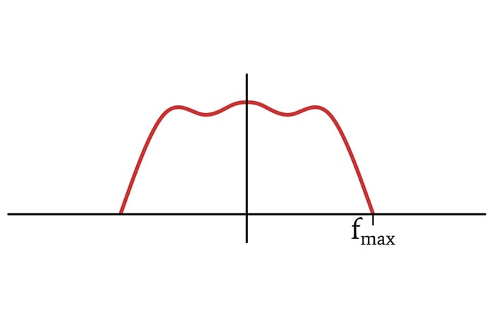
Let’s say that we want to digitize an audio signal that includes a mixture of many different frequencies within a specified range. The high end of the range is defined as f_MAX, and we’ll assume that the range extends down to DC, even though we can’t hear frequencies that low. The Fourier transform of such a signal might look something like this:

Mathematical Sampling in the Time Domain

In the mathematical realm, ideal sampling is equivalent to multiplying the original time-domain waveform by a train of delta functions separated by an interval equal to 1/f_SAMPLE, which we’ll call T_SAMPLE. (For the rest of the article, we’ll use f_S for f_SAMPLE and T_S for T_SAMPLE.) This multiplication causes the sampled signal to be zero between the delta functions and to retain the value of the original signal at each point in time that coincides with a delta function.

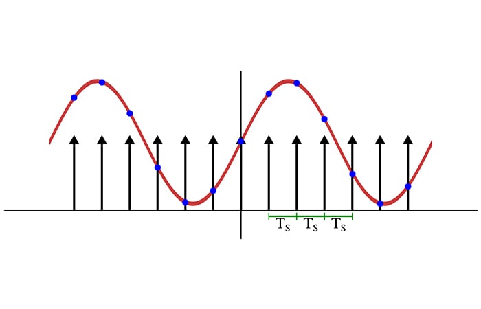
Time-domain sampling implemented mathematically: we multiply the analog signal by a sequence of delta functions occurring at the sampling frequency.

Mathematical Sampling in the Frequency Domain

How does this time-domain sampling procedure affect the frequency-domain representation of a signal? Let’s take a look.

The first thing to remember is that multiplication in the time domain becomes convolution in the frequency domain. Thus, we can find the Fourier transform of the sampled signal by convolving the Fourier transform of the original signal with the Fourier transform of the delta functions.

It turns out that the Fourier transform of a delta-function train is a delta-function train. The difference is that the delta functions are separated by a horizontal distance corresponding to the sampling frequency rather than the sampling period.

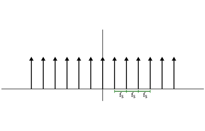
The spectrum of a sequence of delta functions separated by the sampling period is a sequence of delta functions separated by the sampling frequency. 

When we convolve the spectrum of the delta functions with the spectrum of the original signal, we create copies of the original spectrum that are shifted according to the position of the delta functions. Thus, the spectrum of a sampled signal consists of multiple identical “subspectra” that are centered on ±f_S, ±2f_S, ±3f_S, and so on.

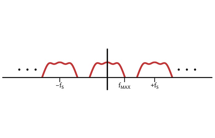
Adequate sampling frequency results in subspectra that are shifted enough to maintain full separation. 

We now have the information we need to confirm the Nyquist–Shannon theorem via frequency-domain analysis. This theorem, as I expressed it in the previous article, is the following:

If a system uniformly samples an analog signal at a rate that exceeds the signal’s highest frequency by at least a factor of two, the original analog signal can be perfectly recovered from the discrete values produced by sampling.

Because of the negative-frequency portion of the Fourier transform, the full mathematical bandwidth of the original signal is 2f_MAX. Thus, in order to ensure that the subspectra do not overlap, we must shift them by at least 2f_MAX. In other words, the sampling frequency must be higher than the signal’s maximum frequency by at least a factor of two.

If this condition is met, the original signal can be perfectly reconstructed. Why? Because the original spectrum has not been altered, and we can eliminate the other subspectra via low-pass filtering. (The next article will explore this point in more detail.) If the condition is not met, the subspectra overlap, the original spectrum is altered, and no amount of low-pass filtering will restore the original signal.

Aliasing

Subspectra overlap is the reason why information is corrupted when we use a sampling frequency that is lower than the Nyquist rate. The overlapping sections of subspectra combine through addition; if we try to separate out the original spectrum using a low-pass filter, the frequency content in the overlapping bands will be different, and consequently the corresponding time-domain signal will be different.

The official name for this is aliasing.

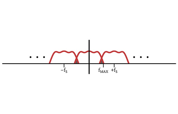
The triangular areas shaded in brown represent aliasing that has caused spectral alteration. 

One of the definitions of the noun “alias” is “a false or assumed identity.” We use the term “aliasing” because this sampling phenomenon can cause one frequency component to shift into a new location in the spectrum and thereby “disguise” itself as a different frequency.

We saw this in the previous article, where sampling at 1.1f_SIGNAL resulted in a discrete-time waveform that appeared to have a frequency much lower than the frequency of the original analog waveform.

Conclusion

At this point, I think that we’ve covered the foundational aspects of sampling theory. In the next article, we’ll start to form some connections between theory and practice.