Understanding Magnetic Field Energy and Hysteresis Loss in Magnetic Cores
In this article, we use the concept of magnetic field energy to explore the relationship between a core's hysteresis loss and its B-H curve.
Magnetic cores are essential components of many electrical and electromechanical devices, including transformers, inductors, motors, and generators. However, some of the energy input to these cores is inevitably dissipated as heat, reducing the efficiency and performance of the devices. The heat generated by these losses can also damage the core material.
One of the main core losses we need to pay attention to, especially at high frequencies, is the hysteresis loss. This is defined as the energy dissipated in a material due to the rotation and alignment of the material’s magnetic domains with the externally applied field.
As you may recall from your college courses, the hysteresis loss of a magnetic core is proportional to the area of the core material’s B-H curve. This article aims to clarify this fundamental relationship. To do so, we first need to develop a solid understanding of how inductors exchange energy with circuits and how energy is stored in a magnetic field.
Magnetic Field Energy: An Overview
Both electric fields and magnetic fields store energy. The concept of energy storage in an electric field is fairly intuitive to most EEs. The concept of magnetic field energy, however, is somewhat less so.
Consider the charging process of a capacitor, which creates an electric field between the plates. It makes sense that accumulating electric charge on the plates of a capacitor requires energy. As more charge accumulates on the plates of the capacitor, the potential difference between the plates increases. If we create a conductive path between the plates, the capacitor releases the stored energy by creating a discharge current through the circuit.
Now consider an inductor. When an inductor is carrying current, it stores energy in a magnetic field. Establishing or increasing the current requires an energy source—a battery, let’s say—to do some work.
To better understand this, we can look to Faraday’s law of induction and Lenz’s law. Faraday’s law tells us that increasing the inductor current will induce an electromotive force (EMF) between the terminals of the inductor. Lenz’s law, as illustrated in Figure 1, tells us that the EMF’s polarity will oppose the change in current.
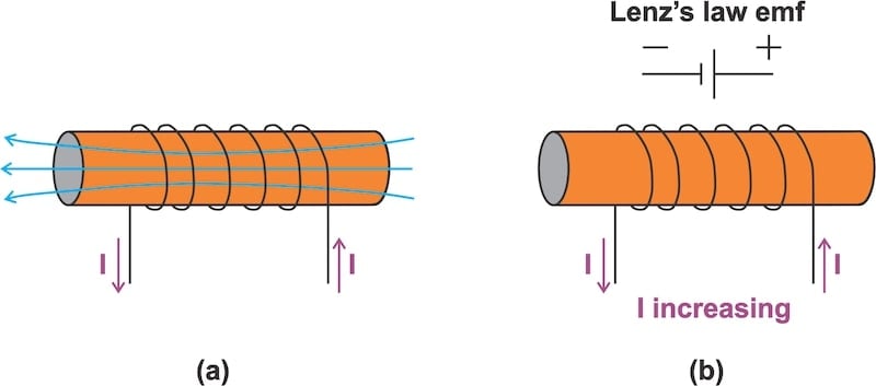
Figure 1. (a) A fixed current in the depicted direction produces a magnetic field directed to the left. (b) When the current is increased, an EMF is induced that tries to oppose a change in the current.
To increase inductor current—and, by extension, the amount of energy stored in the magnetic field—the battery has to do work against the induced EMF. This is analogous to the opposition we face when we try to accumulate charges of the same polarity on a capacitor plate. In both cases, the energy source has to do some work and deliver energy to its load.
Calculating the Magnetic Field Energy
The energy delivered to an inductor with inductance L can be found by using the general instantaneous power equation:
$$P ~=~ v i ~=~ L i \frac{di}{dt}$$
Equation 1.
where v and i are the inductor’s instantaneous voltage and current, respectively.
The incremental energy (dU) supplied to the inductor during an infinitesimal time (dt) is \( dU~=~P~\times~dt\). If we substitute in the value of P from Equation 1, we obtain:
$$dU~=~ L i \; di$$
Equation 2.
Let’s assume that the current of the inductor changes from I1 to I2, where both I1 and I2 are positive values. We can find the energy delivered to the inductor (U) by taking the integral of the above equation, giving us:
$$U ~=~ L \int_{I_1}^{I_2} ~i \; di~=~\frac{1}{2}L \big ( {I_2} ^2 ~-~ {I_1}^2 \big )$$
Equation 3.
The above equation shows how energy storage occurs in an inductor. There are three different scenarios to consider:
- If the inductor current is increased from I1 to I2 (I2 > I1), U is positive. The battery therefore delivers some energy to the inductor.
- If the inductor current is constant (I1 = I2), U is equal to zero. No energy is input to the inductor.
- If the inductor current is reduced from I1 to I2 (I2 < I1), U is a negative value, meaning that the inductor acts as a source that supplies some energy to the external circuit.
Therefore, the energy stored in an inductor with current I is found by substituting I2 = I and I1 = 0 into Equation 3. This leads to:
$$U ~=~ \frac{1}{2}L I^2$$
Equation 4.
What Happens to the Energy in the Inductor?
The energy stored in an inductor can be transferred to other components in a circuit, such as a capacitor or a resistor. For example, consider the circuit in Figure 2.

Figure 2. A theoretical circuit that shows how an inductor releases its initial energy.
This circuit contains two switches, S1 and S2. They operate such that when one switch is closed, the other is open.
Suppose that S1 has remained closed long enough that the current flowing through the inductor has reached its equilibrium value (I = VS/R). We then open S1 and close S2. This connects an inductor with an initial current of I0 = VS/R to the resistor. The current through this RL circuit is a decaying exponential given by:
$$I~=~I_0 e^{-\frac{Rt}{L}}$$
Equation 5.
As current flows through the RL circuit, a power of RI2 is delivered to the resistor. Integrating the power over the limits t = 0 to t = infinity gives us the total energy delivered to the resistor. You can easily verify that the total energy delivered to the resistor is equal to the magnetic field energy that was stored in the inductor at the instant we opened S1 (which is given by Equation 4).
Keep in mind that this is a theoretical example. The whole stored energy is supplied to the circuit because we’re assuming the inductor to be lossless. Due to hysteresis loss—not to mention other loss mechanisms, such as eddy current loss—a real-world inductor will dissipate some of the input energy as heat. A little later on, we’ll see how the hysteresis loss manifests itself in the B-H curve of the inductor’s core material.
Magnetic Energy in Terms of Field Quantities
It’s helpful to write the magnetic field energy in terms of the magnetic flux density (B) and magnetic field intensity (H). The volume energy density required to change the magnetic field from B1 to B2 is:
$$w_m ~=~ \int_{B_1}^{B_2} H~\times~ dB$$
Equation 6.
Proving the above equation in its general form is rather complicated. However, for simple structures such as solenoids or toroidal coils, we can derive Equation 6 by applying a similar procedure to what we used in Equation 3. Let’s examine a solenoid.
Magnetic Energy Density of a Solenoid
Consider a solenoid that uses a magnetic core. The solenoid has N turns and a length of l; the hysteresis loop of its core is shown in Figure 3.

Figure 3. The hysteresis loop of an example solenoid’s magnetic core.
If the solenoid’s initial magnetic field intensity is h1, what is the energy required to increase the flux density by ΔB?
Our first step is to find the instantaneous power delivered to the inductor during an infinitesimally small time (Δt):
$$P ~=~ vi ~=~ i \Big ( N \frac{\Delta \Phi}{\Delta t} \Big )$$
Equation 7.
This is the same equation as Equation 1, except that the inductor voltage is now expressed in terms of the magnetic flux (ɸ) through the cross-sectional area of the coil. If the cross-sectional area is A, we have \(\Delta \Phi~=~A~\times~\Delta B\), which then leads to:
$$P ~=~ i N A \frac{\Delta B}{\Delta t}$$
Equation 8.
For a solenoid with N turns and length l, the magnetic field intensity is H = Ni/l. Assuming that Point A in Figure 3 corresponds to a current of i1 and field intensity of h1, Equation 8 can be rewritten as:
$$P ~=~ lA ~\times~ h_1 \frac{\Delta B}{\Delta t}$$
Equation 9.
The incremental energy (ΔU) supplied to the inductor during the time interval Δt is:
$$\Delta U~=~P~\times~\Delta t$$
Equation 10.
which results in:
$$\Delta U ~=~ lA ~\times~ h_1 ~\times~\Delta B$$
Equation 11.
Finally, noting that lA is the volume of the solenoid, the incremental energy density delivered to the inductor is h1 × ΔB. This is consistent with Equation 6.
Referring back to Figure 3, we see that the delivered energy density (h1 × ΔB) is equal to the area of the shaded strip. This is the key observation we need to calculate hysteresis loss.
Calculating the Hysteresis Loss of a Solenoid
When a sinusoidal magnetic field is applied to a ferromagnetic material, some energy is dissipated in the material due to the resulting rotation and alignment of its magnetic domains. Given that, how much energy is needed to maintain a sinusoidal magnetic field in the material?
Let’s consider a full cycle around the hysteresis loop in Figure 3, starting from Point f and following the path fgbcdef back to Point f. As we move from Point f to Point g to Point b on the hysteresis curve, the energy density required to change the magnetic flux density is equal to the integral of (H × dB) over this path. The result of this integral (Equation 6) is equal to the cyan area in Figure 4.

Figure 4. Energy delivered to the inductor going from Point f to Point b.
The current increases along the path fgb. Energy is therefore delivered to the inductor. Another way to understand this is by noting that both H and db (or, equivalently, ΔB in short successive time intervals) are positive as we move from f to b. That tells us that the delivered energy is positive.
Next, let’s consider the path from b to c. Again, the energy exchanged between the inductor and the external circuit is proportional to the area between the hysteresis curve and the B-axis. In Figure 5, this area is colored magenta.

Figure 5. Energy supplied by the inductor going from Point b to Point c.
The magenta area in the figure shows the energy supplied by the inductor, not the energy received by it. H is reduced over this part of the curve, and thus so is the inductor current. The inductor is supplying power to the external circuit. We could also reach the same conclusion by noting that in this case H is positive and dB is negative, meaning that the energy delivered to the inductor is negative.
The net energy density delivered to the inductor as we follow the path fgbc is found by subtracting the magenta area in Figure 5 from the cyan area in Figure 4. This leaves us with the purple area in Figure 6.

Figure 6. The net energy delivered to the inductor when going from Point f to Point c along the path fgbc.
Similarly, the energy for the path cde corresponds to the cyan area in Figure 7, and the energy for the path ef to the magenta area in Figure 8.

Figure 7. Energy delivered to the inductor going from Point c to Point e.

Figure 8. Energy supplied by the inductor going from Point e to Point f.
Once again, the cyan area shows the energy delivered to the inductor and the magenta area corresponds to the energy supplied by the inductor. The net energy density delivered to the inductor as we follow the path cdef is found by subtracting the magenta area from the cyan area, leading to the purple area in Figure 9.

Figure 9. The net energy delivered to the inductor when going from Point c to Point f along the path cdef.
Taken together, Figures 6 and 9 show the total energy density required to maintain one cycle of a sinusoidal magnetic field in a ferromagnetic material. This energy, which is dissipated in the material as heat, is equal to the area enclosed by the hysteresis loop. The larger the area of the hysteresis, the more loss there is per cycle.
We can estimate the hysteresis loss of different materials simply by using this key observation. We’ll discuss this at greater length in the next article of this series, which will also introduce an empirical method of finding the hysteresis loss in a magnetic core.
All images used courtesy of Steve Arar