Understanding Digital Oscilloscope Sample Rate and Analog Bandwidth Specs

In this article, we’ll examine two important specifications of a digital oscilloscope: analog bandwidth and sampling rate. We’ll see that the scope analog bandwidth determines whether or not we can accurately measure a signal with a given frequency. Moreover, we’ll discuss that a sufficiently high sampling rate is required to avoid aliasing which can reduce the measurement accuracy as well. 

 

Simplified Block Diagram of an Oscilloscope

Figure 1 shows a simplified block diagram for a digital oscilloscope. 

 

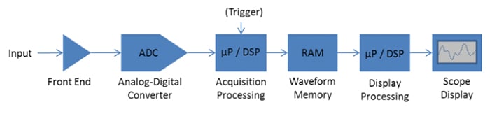
Figure 1. Image courtesy of Tektronix.

 

The analog front end attenuates/amplifies the input signal and acts as an anti-aliasing filter for the A/D converter (ADC). The conditioned input is sampled by the ADC at a fixed sample rate f_s and the digitized samples are passed on to the trigger system. The main purpose of the trigger system is providing a stable display of the waveform. It determines which samples should be displayed on the screen. These samples are stored in memory and processed before being displayed on the screen.   

 

Oscilloscope Analog Bandwidth

The analog front end consists of blocks such as the gain control circuitry, buffers, and ADC drivers. These blocks exhibit a low-pass frequency response. The frequency at which the amplitude of the transfer function is attenuated by 3 dB is considered the analog bandwidth f_BW of the scope. This is illustrated in Figure 2.

 

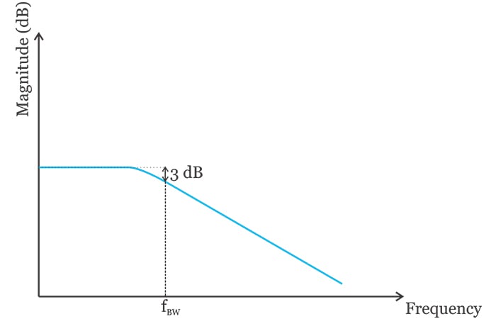
Figure 2

 

What frequency range can be processed by an oscilloscope with analog bandwidth of f_BW?

To answer this question, we note that our measurement device should not cause undesirable modifications in the signal to be measured. For example, we shouldn’t use the above oscilloscope to measure a sinusoid with frequency f_BW because such a signal will be attenuated by 3 dB as it goes through the low-pass filter. In this case, the scope will digitize and display the attenuated version which is not desired. Therefore, the frequency range with minimal attenuation is the useful bandwidth of the scope.

 

Measuring Analog Signals  

As long as we remain below approximately one-third of the scope bandwidth \(\left (\frac{f_{BW}}{3} \right )\), we can assume that the scope transfer function has negligible attenuation. Therefore, when measuring analog signals, we should make sure that the maximum signal frequency is less than \(\frac{f_{BW}}{3}\). This rule of thumb is based on the assumption that the scope frequency response is almost flat in the pass-band of the transfer function.

With some low-cost oscilloscopes, particularly those manufactured by small companies, the frequency response might not be flat. If we are not sure about the scope frequency behavior, we can measure it by applying a frequency-swept test sinusoid and examining the amplitude of the displayed waveform. 

 

Measuring Digital Signals

What about measuring a digital waveform? What is the maximum clock frequency that can be measured by an oscilloscope with analog bandwidth f_BW? In a previous article, we discussed that the frequency content of a digital waveform depends on its rise/fall time. For a signal with rise time T_r, we can define an equivalent bandwidth given by:

 

\[BW_{clock}=\frac {0.35}{T_r}\]

 

In this equation, T_r is the 10-90% rise time of the digital signal. For example, for a clock signal with T_r = 0.5 ns, the equivalent bandwidth will be 700 MHz. This means that the highest significant frequency component of this waveform is below about 700 MHz. Please refer to the article I mentioned above to learn about the meaning of “significant” in this context.

We assumed that the scope transfer function has negligible attenuation below \(\frac{f_{BW}}{3}\). Therefore, the highest significant frequency component of the digital waveform should be less than about \(\frac{f_{BW}}{3}\):

 

\[\frac {0.35}{T_r}= \frac{f_{BW}}{3}\]

 

We obtain:

 

\[f_{BW}=\frac {1.05}{T_r}\]

Equation 1 

 

For example, the scope bandwidth for measuring a digital signal with T_r=500 ps is about f_BW=2.1 GHz. The topic of choosing the correct scope bandwidth for a particular measurement is discussed in a Keysight application note in greater detail. The equation we derived here is close to the one the application note gives for a 3% accurate measurement using a Gaussian response oscilloscope:

 

\[f_{BW}=\frac {0.95}{T_r}\]

 

The Keysight application note gives slightly different equations for different scenarios but you can use Equation 1 as a simplified general equation to assess the scope bandwidth when measuring a digital signal.

 

The Disadvantage of Excessive Scope Bandwidth

The scope bandwidth should be high enough to make accurate measurements, but is there an upper limit for this parameter? Can excessive scope bandwidth degrade our measurement accuracy in some way? Note that the scope bandwidth sets the bandwidth of the noise that enters the oscilloscope.

As an example, consider measuring a 33 MHz sinusoid. Based on the above discussion, we can use a scope with bandwidth of about 100 MHz to measure this signal. If we use an 8 GHz oscilloscope for this measurement, all of the noise components that reside in the range from 100 MHz to 8 GHz will enter the scope. These noise components will make the trace look a bit blurry on the screen.

This might not be a serious problem in many cases, but if you want your product to pass strict performance or compliance specs, you have to pay attention to these details and provide the best presentation of your product output. 

 

Sampling Rate

After the input signal is conditioned by the analog front end, it is passed on to the A/D converter. According to the Nyquist Sampling Theorem, the sampling rate of the ADC f_s must be at least twice the highest frequency component of interest. This means we need an anti-aliasing filter to restrict the bandwidth of the signal at the ADC input. In Figure 1, the anti-aliasing filtering is achieved by the low-pass characteristic of the analog front end.

Although the high-frequency components are suppressed by this filter, we don’t have a brick-wall low-pass characteristic. As we move to higher frequencies, the magnitude attenuation increases but we don’t have infinite attenuation. Assume that we choose the sampling frequency f_s as shown in Figure 3. 

 

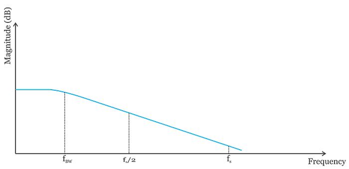
Figure 3

 

Since we have limited attenuation at f_s, any noise component that appears at this frequency will be only partially suppressed by the low-pass characteristic. In other words, the bandwidth of the signal at the ADC input is not really limited and we might still have relatively large frequency components above \(\frac{f_s}{2}\)(Nyquist criterion violation).

How is this going to affect the accuracy of our measurement?

The sampling process will create replicas of the spectrum at multiples of the sampling frequency. In the frequency range from 0 to f_s, we’ll have the spectrum shown in Figure 4. 

 

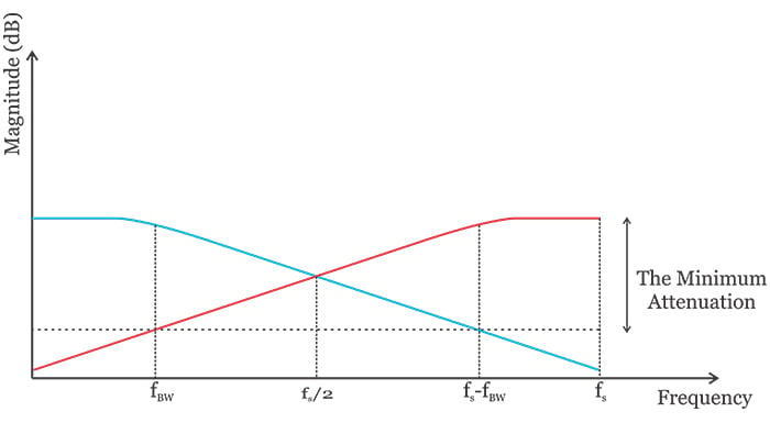
Figure 4

 

While the blue curve is the spectrum we wanted at the output of the digitizer, an undesired replica of the original spectrum (depicted by the red curve) is created by the sampling process. A superposition of the components from both the blue and red curves gives us the spectrum of the digital signal at the ADC output.

Figure 4 shows that part of the replica spectrum has overlap with our desired frequency band that resides in the range from 0 to f_BW. This desired frequency band should be extracted and processed by the digital circuitry that follows the A/D converter. How can we extract this desired frequency band? 

The frequency components from f_BW to f_s-f_BW can be efficiently suppressed by a sharp digital filter (See Figure 5). Eliminating this unwanted frequency band leads to a more efficient digital circuitry. 

 

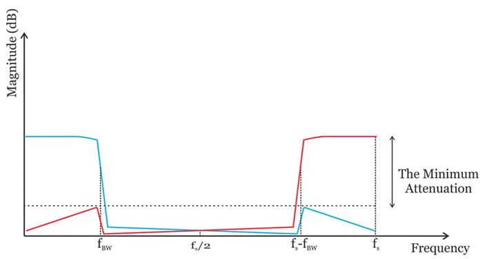
Figure 5

 

What about the part of the replica spectrum that shows up in the 0-to-f_BW range?

These frequency components cannot be suppressed by placing a filter at the output of the ADC. As shown in Figure 4, these undesired components are folded back from the part of the original spectrum that resides in the range from f_s-f_BW to f_s. Hence, we can suppress these aliased components by increasing the sampling rate (for a given f_BW). In this way, the minimum attenuation that the aliased components will experience increases.

Check out Figure 4. What is the minimum acceptable attenuation for the folded-back components?

The attenuation should be large enough to bring the aliased components to well below the quantization level of the A/D converter. In practice, with a Gaussian frequency response oscilloscope, we usually need the real-time sampling rate to be 4-5 times the oscilloscope bandwidth. Oscilloscopes with a maximally-flat frequency response have a sharper roll-off. As a result, a sampling rate of about 2.5 times the oscilloscope bandwidth leads to an acceptable accuracy with this type of oscilloscope.

How would the displayed trace be affected if the aliasing is significant?

Figure 6 shows a measurement where the oscilloscope bandwidth and sampling rate are 500 MHz and 1 GSa/s, respectively.

 

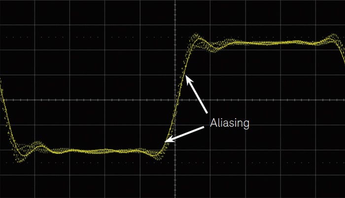
Figure 6. Image courtesy of Keysight.

 

As you can see, the trace wobbles around the signal edge when repetitive measurements are made. This is due to the fact that the parts of the waveform that have sharper transitions incorporate higher frequency components and aliasing becomes more significant in these regions. 

 

Conclusion

In this article, we looked at two important specifications of a digital oscilloscope: analog bandwidth and sampling rate. We saw that, with an analog signal, the maximum signal frequency should be less than about \(\frac{f_{BW}}{3}\).

For measuring a digital signal, we can restrict the highest significant frequency component of the digital waveform to less than about \(\frac{f_{BW}}{3}\). Moreover, we discussed that a sufficiently high sampling rate is required to avoid aliasing.

With a Gaussian frequency response oscilloscope, we usually need the real-time sampling rate to be 4-5 times the oscilloscope bandwidth. Oscilloscopes with a maximally-flat frequency response have a sharper roll-off and a sampling rate of about 2.5 times the oscilloscope bandwidth should be sufficient.

To see a complete list of my articles, please visit this page.