Understanding Cutoff Frequency in a Nyquist Plot

This article continues our exploration of the Nyquist plot by examining the relationship between the plot’s curve and a filter’s cutoff frequency.

In a previous article, we saw that the frequency response of a system can be represented by a polar plot whose curve indicates magnitude and phase as frequency varies from zero to infinity. We call this a Nyquist plot (or Nyquist diagram), and it’s an interesting alternative to the much more common Bode plot.

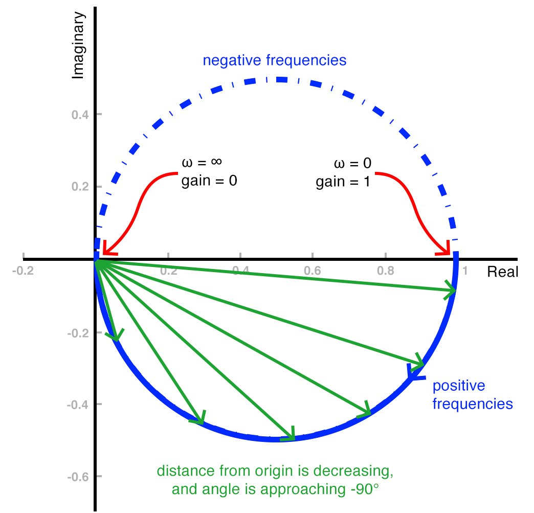
The following diagram was presented at the end of the preceding article, and it provides a good visual summary of the general information that we can extract from the Nyquist plot of a first-order filter.

 

 

 

The Importance of the Cutoff Frequency

The above diagram doesn’t include one very important piece of information, namely, the filter’s cutoff frequency. The s-domain transfer function of a first-order low-pass filter can be expressed as follows:

 

$$T(s)=\frac{K}{1+(\frac{s}{\omega _{O}})}$$

 

This equation tells us that the only distinguishing characteristics of a given low-pass filter are K and ω_O. The parameter K is the filter’s low-frequency gain. Passive components have no ability to amplify a signal, so if we’re concerned only with RC first-order low-pass filters, we can ignore K, because it will always be 1. The remaining parameter, ω_O, is the cutoff frequency. Thus, we can fully describe an RC low-pass filter simply by specifying the cutoff frequency.

Finding the Cutoff Frequency

A Nyquist curve certainly doesn’t have the typical roll-off characteristic that we know so well from Bode plots, and in fact, a Nyquist plot does not give us specific information about the cutoff frequency of a filter circuit. However, examining the relationship between cutoff frequency and a Nyquist curve is a good way to reinforce the concept of cutoff frequency in general, and it also will give us some insight into the limitations of the Nyquist approach to visually depicting frequency response.

First, we need to think about what is actually happening at the cutoff frequency, with respect to both magnitude response and phase response.

 

Cutoff Frequency via Magnitude

You probably know that another name for the cutoff frequency is the 3 dB (or –3 dB) frequency, and this reminds us that a first-order low-pass filter provides 3 dB of attenuation (or, equivalently, –3 dB of gain) when the input frequency is ω_O. We don’t use decibels in a Nyquist plot, so instead of –3 dB, we use the corresponding amplitude ratio, which is $$\frac{1}{\sqrt{2}}$$.

When we’re working with a polar plot, we should always be mindful of triangles; for example, the magnitude of a complex number is determined as though it is the hypotenuse of a right triangle whose two legs are the real and imaginary components, and we use trigonometry to calculate the angle of a complex number. Now that you’re thinking in terms of triangles, does the factor $$\frac{1}{\sqrt{2}}$$ give you any ideas?

 

 

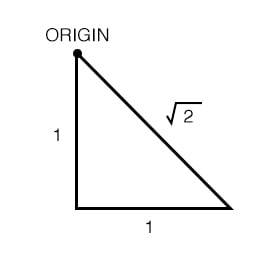
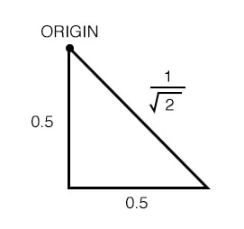
As shown above, the factor $$\sqrt{2}$$ comes into play whenever a right triangle has two legs of equal length. If we reduce the length of the legs to 0.5, the length of the hypotenuse is $$\sqrt{2}$$ × 0.5, which is the same as $$\frac{1}{\sqrt{2}}$$.

 

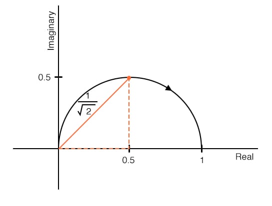
So what does all this mean? Consider the following Nyquist plot:

 

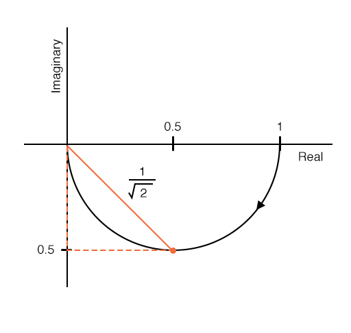
This is the Nyquist plot for a first-order low-pass filter. Note that I did not include the portion of the curve that corresponds to negative frequencies.

 

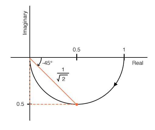
As you can see, the filter has a gain of $$\frac{1}{\sqrt{2}}$$ at the lowest point of the curve, where the absolute value of the real component is equal to the absolute value of the imaginary component, and this is the location of the cutoff frequency in the Nyquist plot of a first-order low-pass filter. The same relationship applies to a first-order high-pass filter, except that in this case, the cutoff frequency is at the highest point of the curve:

 

 

The difference is due to the fact that the high-pass filter’s phase shift varies from +90° to 0° as frequency increases, whereas the low-pass filter’s phase varies from 0° to –90°. Because the angle is measured counterclockwise from the positive real axis, positive phase shift is plotted above the real axis and negative phase shift is plotted below the real axis.

Note also that the two plots have arrows pointing in opposite directions: in the low-pass plot, the arrow points toward the origin because gain decreases as frequency increases; in the high-pass plot, it points away from the origin, because gain increases as frequency increases.

Cutoff Frequency via Phase Shift

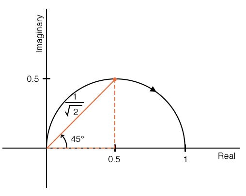
We can also find the cutoff frequency in a Nyquist plot if we recall that the 90° of phase shift produced by a first-order filter is centered on the cutoff frequency. In other words, the phase shift at ω_O is +45° or –45°. A vector drawn in the complex plane will have an angle of +45° or –45° when its real and imaginary parts have equal absolute value, and this leads us to the same geometrical relationship that we found when considering cutoff frequency from the perspective of magnitude response.

 

 

 

 

Summary of Cutoff Frequencies in Nyquist Plots 

You may have noticed that the location of the cutoff frequency in these Nyquist plots is purely geometrical. You can’t attach a fixed frequency value to the location, since the location is the same for every first-order low-pass filter or for every first-order high-pass filter. The Nyquist plot is clearly not a replacement for Bode plots; however, it is a more direct way to convey information about a system’s transfer function, and as we’ll see in a future article, it’s a handy tool in stability analysis.