Understanding Butterworth Filter Poles and Zeros

Many people have heard the term “Butterworth filter” and have used these types of filters in their circuits. You certainly don’t have to be an expert in filter theory to successfully incorporate a filter topology into your designs. However, in some cases, it is beneficial to understand things more thoroughly. In the days of SPICE and Google searches and filter calculators, we sometimes need to take a step back and think about the theoretical and conceptual foundation upon which a functional circuit is built.

My objective in this article is to help you understand the Butterworth filter by presenting and discussing aspects of its pole-zero diagram.

 

Poles and Zeros

I previously wrote an article on poles and zeros in filter theory, in case you need a more extensive refresher on that topic. Poles represent frequencies that cause the denominator of a transfer function to equal zero, and they generate a reduction in the slope of the system’s magnitude response. Zeros represent frequencies that cause the numerator of a transfer function to equal zero, and they generate an increase in the slope of the system’s transfer function.

In this article, we will focus on the Butterworth low-pass filter, which has at least two poles and no zeros. (All low-pass filters have at least one zero at ω = infinity, but these don’t appear in the pole-zero diagram and can usually be ignored.)

 

Plotting Poles and Zeros

Information about a system’s poles and zeros can be conveyed visually by marking their locations in the complex plane. If you’ve read my article on the Nyquist plot or on complex-conjugate poles, or Dr. Sergio Franco’s article on pole splitting, you are familiar with the concept of a pole-zero plot.

The following diagram demonstrates the basic structure.

 

         

 

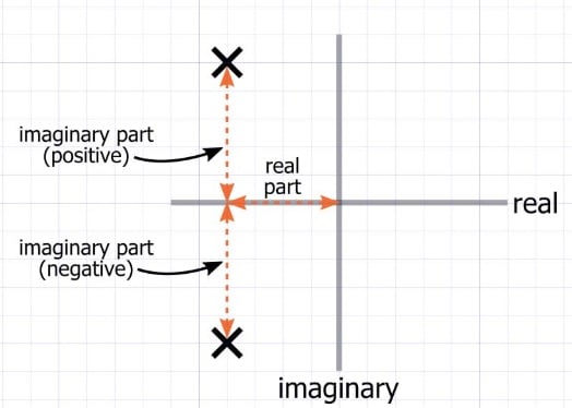
The location of a pole or zero is determined by its real part, which is plotted horizontally, and its imaginary part, which is plotted vertically. Poles are marked with an ✕, and zeros are marked with a circle. In the example above, the two poles represent a complex-conjugate pair, because they have real parts that are equal and imaginary parts that are equal in magnitude but opposite in sign.

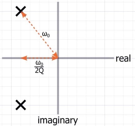
A pole-zero plot is a convenient and effective means of conveying important information about a filter system. As you can see in the diagram below, it indicates both pole/zero frequency and Q factor:

 

    

The Butterworth Topology

I use the word “topology” here to emphasize the fact that the Butterworth “filter” is actually a class of circuits that have the same general characteristics.

As with most other things in life, you can’t have one system or device or material that is better than all others in every way. Instead, we have trade-offs: performance vs. affordability, durability vs. weight, free time vs. back-account balance, and so forth.

The Butterworth priority is passband flatness, and that is what unites the various instantiations of the Butterworth topology: they minimize the amount of magnitude variation that occurs prior to the cutoff frequency. This contrasts with the Chebyshev topology, which allows passband ripple in order to increase the steepness of the transition from passband to stopband.

Passband flatness is evident in the following plot, which is the magnitude response of a fourth-order Butterworth filter.

 

 

The Butterworth Pole-Zero Plot

To achieve a low-pass Butterworth response, we need to create a transfer function whose poles are arranged as follows:

 

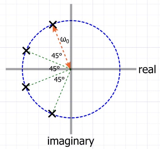
This particular filter has four poles. Additional poles would need to follow the same pattern.

 

The following bullet points will help you to unpack the information contained in this diagram.

• The fundamental characteristic of a low-pass Butterworth pole-zero plot is that the poles have equal angular spacing and lie along a semicircular path in the left half-plane.
• All points on a circle have the same distance from the center of the circle. Thus, the distance between the origin and each pole is the same, and this in turn means that all poles have the same frequency.
• The angle that separates the poles is equal to 180°/N, where N is the order of the filter. In the example above, N = 4, and the separation angle is 180°/4 = 45°.
• The equal angular spacing of the Butterworth poles indicates that even-order filters will have only complex-conjugate poles. Odd-order filters have complex-conjugate poles plus one purely real pole that lies along the negative real axis at a distance of ω0 from the origin.
• All poles have the same \[ω_0\], but the horizontal distance from the origin varies. Thus, the poles have different Q factors.

 

Conclusion

The pole-zero diagram that we examined in this article is not simply a way to describe a low-pass filter. Rather, the pole configuration is the theoretical basis for the design of a Butterworth filter. Given the required cutoff frequency and filter order, we would choose components such that pole locations adhere to the Butterworth arrangement.

Translating from pole-zero diagram to component values is not particularly easy; precalculated tables were used in the days before handy software tools, and my guess is that you’ll never need to perform this process manually. Nonetheless, it’s good to know at least something about underlying concepts, and I hope that you enjoyed this discussion of Butterworth theory.