How to Analyze Transmission Line Transformers: The Easy Way and the Hard Way

By using transmission lines in place of windings, transmission line transformers are able to operate at high frequencies and across wide bandwidths. As we learned in an earlier article, these capabilities make them very useful in RF and microwave applications. However, beginners often find transmission line transformers confusing to analyze.

In this article, we’ll try to remove some of that confusion by walking through each of the two common methods for transmission line transformer analysis. The first method we’ll examine—the “hard way” of the article’s title—provides a greater level of accuracy at the cost of more time spent doing math. The second method provides a simplified analysis that will usually—but not always—be sufficient. Before taking the easy way, it’s important to understand the hard way.

 

The Hard Way: Using Transmission Line Equations

Transmission line transformers rely on electromagnetic wave propagation through a transmission line to transfer energy to the output. A rigorous analysis should therefore consider the transmission line equations. For example, Figure 1 shows a phase inverter circuit built with a bifilar coil.

 

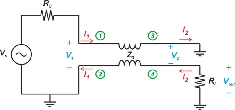
Figure 1. A broadband phase inverter built with a bifilar coil.

 

To analyze this circuit, we’ll use the ABCD parameters of the transmission line to describe the relationship between the input and output ports of the line. Consider the lossless transmission line in Figure 2, which has a characteristic impedance of Z₀, a phase constant of β, and a length of l.

 

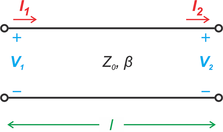
Figure 2. A transmission line with characteristic impedance Z₀, phase constant β, and length l.

 

The ABCD representation of the transmission line describes the voltage and current quantities at the input and output ports through the following equations:

$$V_{1} ~=~ \cos(\beta l) V_{2} ~+~jZ_{0} \sin(\beta l) I_{2}$$

Equation 1.

 

$$I_1 ~=~j\frac{\sin(\beta l)}{Z_0} V_2 ~+~ \cos(\beta l) I_2$$

Equation 2.

 

These are the main two equations we’ll use to analyze the phase inverter circuit. We’ll also obtain an additional equation from Figure 1 to relate the output voltage and current:

$$V_2 ~=~ R_L I_2$$

Equation 3.

 

where R_L is the load resistance.

Assuming a matched load (Z₀ = R_L), we can use some algebra to combine Equation 3 with Equation 1. This gives us the relationship between the input and output voltages:

$$V_{2}~=~e^{-j \beta l}V_{1}$$

Equation 4.

 

As this equation demonstrates, the amplitude of the signal along the transmission line is constant for a matched load. The line only introduces a phase shift to the input signal.

The final output voltage is calculated as:

$$V_{out}~=~-V_{2}~=~-e^{-j \beta l}V_{1}$$

Equation 5.

 

This shows that the circuit acts as a phase inverter if the phase shift from the exponential term is negligible. For the transfer function to exhibit a 180 degree phase shift, we should have \( \beta l ~\ll~ 1 \). Recall that the phase constant β is given by:

$$\beta ~=~ \frac{2 \pi}{ \lambda }$$

Equation 6.

 

Therefore, in order to ignore the phase shift from the exponential term, the length of the line should satisfy the following constraint:

$$l ~\ll~ \frac{\lambda}{2 \pi}$$

Equation 7.

 

To summarize, two conditions must be met for the circuit to act as a phase inverter:

• The loss of the line must be negligible.
• The length of the line must be short enough for the phase shift from the exponential term to be ignored.

This method, though accurate, is relatively math-intensive. Let’s discuss a more intuitive way to determine the circuit’s impedance transformation ratio.

 

The Easy Way: The Lumped Inductor Method

When it comes to analyzing impedance transformation, many books assume that the transmission line transformer behaves similarly to a magnetically coupled transformer. This assumption allows us to avoid the complex math we saw in the preceding section. For example, let’s see what happens if we analyze the phase inverter circuit—reproduced in Figure 3 for ease of reference—as if it were a magnetically coupled transformer.

 

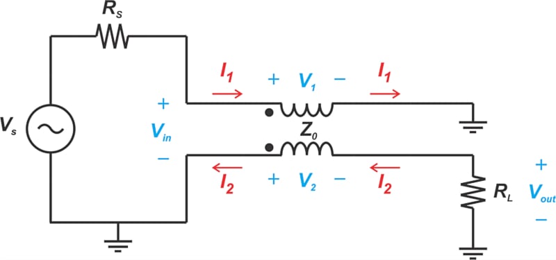
Figure 3. Analyzing the broadband phase inverter as a conventional transformer.

 

In this case, we assume that the voltage across the primary winding (V₁) is also impressed across the secondary winding (V₁ = V₂). Likewise, the same current flows through the primary and secondary windings. To find the polarity of the voltages and the direction of the currents, we apply the transformer dot convention to the figure above. Applying Kirchhoff’s voltage law, we obtain:

$$V_{out}~=~-V_2 ~-~ V_{in} ~+~ V_1 ~=~ - V_{in}$$

Equation 8.

 

which is consistent with the more precise mathematical analysis we conducted previously.

When applied correctly, the simplified method will provide the same impedance transformation ratio as the more rigorous analysis. For that reason, many references only present the simplified analysis. However, this method relies on us making certain assumptions about the circuit’s behavior—in particular, that the current leaving a winding is the same as the current that entered it.

This is the type of analysis we use with a lumped inductor. For us to assume that the windings of a transmission line transformer act as lumped inductors, the following two statements must be true:

1. The circuit is operating at a low frequency.
2. The transmission line is short relative to the wavelength.

Because a transmission line transformer can act as a magnetically coupled transformer over a considerable portion of its frequency range, the simplified analysis is valid as long as both of the above conditions are met. At high frequencies, however, we should use the transmission line equations to gain a thorough understanding of the circuit’s behavior. The transmission line analysis assumes that the windings act as distributed elements, leading to the assumption that the current entering a winding is different from the current leaving the other end.

 

Wrapping Up

In this article, we learned about two different ways of analyzing a transmission line transformer. Future articles in this series will put that knowledge to use—we’ll use both of the analysis techniques introduced here to examine the Ruthroff class of transformers. Until then, I hope you’ve found today’s discussion informative.

 

All images used courtesy of Steve Arar