Thermocouple Basics—Using the Seebeck Effect for Temperature Measurement
Learn about the Seebeck effect and how the Seebeck voltage and Seebeck coefficient come into play within the scope of thermocouples and temperature measurement.
Thermocouples are a popular type of temperature sensor due to their ruggedness, relatively low price, wide temperature range, and long-term stability. The Seebeck effect discussed in the previous article is the underlying principle that governs the thermocouple operation. The Seebeck effect describes how a temperature difference (ΔT) between the two ends of a metal wire can produce a voltage difference (ΔV) across the length of the wire. This effect is characterized by the following equation:
$$S = \frac{\Delta V}{\Delta T} = \frac{V_{cold}-V_{hot}}{T_{hot}-T_{cold}}$$
Equation 1.
Where S denotes the Seebeck effect of the material. This equation can be also expressed as:
$$S(T)=\frac{dV}{dT}$$
Equation 2.
Here, S(T) emphasizes that the Seebeck effect is a function of temperature. Note that the Seebeck effect is also observed in metal alloys and semiconductors. Let’s see how this effect can be used to measure temperature.
Seebeck Effect of an Individual Material: Copper Wire Example
Equation 1 suggests that by having the Seebeck coefficient of a material, the voltage difference across a conductor can be used to determine the temperature difference between the two ends. Although this is theoretically correct, the direct measurement of an individual material's Seebeck voltage is impossible. As an example, consider the setup shown in Figure 1.
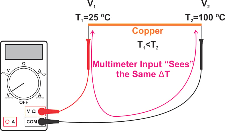
Figure 1. An example setup to measure the voltage across a copper wire.
The ends of the copper wire are at T1 = 25 °C and T2 = 100 °C. Assume that, over this temperature range, the absolute Seebeck coefficient of copper is constant and equal to +1.5 μV/°C. Using Equation 1, we can find the voltage difference across the wire as:
$$V_{1}-V_{2}=1.5\times(100-25)=112.5\,\mu V$$
The voltage measured by the multimeter will be different because the path consisting of the multimeter leads and the input circuitry of the multimeter also experiences a temperature difference of 75 °C. Unwanted Seebeck voltage across the test leads and the input circuitry of the multimeter introduces errors.
Avoiding Seebeck Voltage—Keeping the Multimeter at Uniform Temperature
To avoid creating a Seebeck voltage in the test leads and the multimeter, we should keep these parts at a constant temperature. For example, we can keep the measurement system at 25 °C as shown in Figure 2.
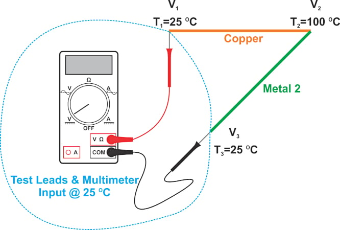
Figure 2. An example setup showing a constant temperature of 25 °C.
In this example, another conductor is required to make the electrical connection between the black test lead and the hot end of the copper wire. This connection is shown by “Metal 2” in the figure. It is important to note that copper wire cannot be used for this connection. This is because it will also experience the same temperature gradient as the original copper wire, leading to a voltage difference (across Metal 2) of:
$$V_{3}-V_{2}=1.5 \times (100-25) = 112.5\,\mu V$$
Therefore, the multimeter will measure zero volts regardless of the temperature difference across the original copper wire. The above discussion shows why the absolute Seebeck coefficient of a material cannot be directly measured by a multimeter. A common method to determine the absolute Seebeck coefficient is by applying the Kelvin relation.
Thermoelectric Thermometry Requires Dissimilar Materials
From the above discussion, it can be surmised that materials with unequal Seebeck coefficients are required to produce a voltage difference proportional to the temperature gradient. For example, with copper that has a Seebeck coefficient of +1.5 μV/°C at 0 °C, we can use a constantan wire with an absolute Seebeck coefficient of -40 μV/°C at 0 °C. Replacing “Metal 2” with a constantan wire, the multimeter should measure a voltage difference of 3112.5 μV, as calculated below:
$$V_{1}-V_{3}= (V_{1}-V_{2})-(V_{3}-V_{2})= 1.5 \times(100-25)-(-40)\times(100 - 25) = 3112.5\,\mu V$$
Note that the above calculation assumes that the Seebeck coefficients of copper and constantan are constant and equal to the specified values over the temperature range of interest.
Thermocouple Temperature Sensor—Thermocouple Types and the Seebeck Coefficient
Therefore, two dissimilar conductors soldered or welded together at one end can be used to create a temperature sensor. The structure of this temperature sensor, known as a thermocouple, is shown in Figure 3.
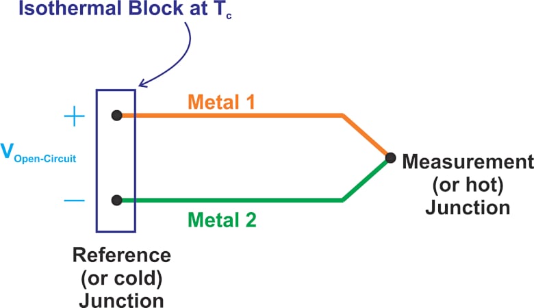
Figure 3. An example structure of a thermocouple temperature sensor.
The junction at which the two dissimilar metals are coupled is called the measurement (or the hot) junction. The opposite end where the sensor connects to the measurement system is called the reference (or the cold) junction. An isothermal block, which is made of a heat conducting material, is commonly required to keep the leads of the thermocouple at the same temperature.
Note that a thermocouple measures the temperature difference between the measurement and reference junctions, not the absolute temperature at these junctions. The open-circuit voltage at the reference junction is proportional to the temperature difference between the two ends.
A thermocouple created by joining a copper wire to a constantan wire is known as a type T thermocouple. Other common thermocouple types are:
- J (iron-constantan)
- K (chromel-Alumel)
- S (Platinum (10%)/Rhodium–Platinum)
Manufacturers commonly specify a thermocouple type's overall Seebeck coefficient (or sensitivity) as a table, graph, or equation. For example, the Seebeck coefficient of a T-type thermocouple at 0 °C is usually specified to be about 39 µV/°C which is close to the value we obtained above from the individual employed metals/alloys (41.5 µV/°C). We know that this sensitivity value changes with temperature. Figure 4 shows the Seebeck coefficient of T-, J-, and K-type thermocouples versus temperature.
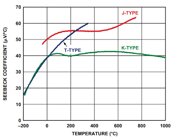
Figure 4. The Seebeck coefficients for T, J, and K type thermocouples vs. temperature. Image used courtesy of Analog Devices
The above curves are obtained with a reference junction at 0 °C. In the next article, we’ll discuss the setup for these measurements in greater detail and see how this information can be used in practice.
Thermocouple Misconceptions Concerning Seebeck Voltage
Although most engineers are familiar with thermocouples, there are a few common misconceptions. Since thermocouples use two dissimilar metals joined at one end to measure temperature, a frequently held misconception is that the Seebeck voltage is produced as a result of joining dissimilar metals. We now know that a single conducting material can produce a Seebeck voltage when there is a temperature gradient.
It’s also important to remember that the Seebeck voltage is not produced at the junction of two dissimilar metals. The Seebeck voltage is developed along the length of the wire that experiences a temperature difference (Figure 5).
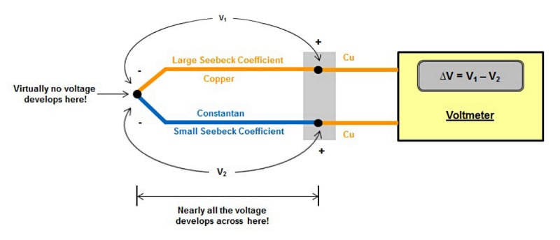
Figure 5. Setup showing the Seebeck voltage across two dissimilar metals. Image used courtesy of TI
The junction provides an electrical connection between the dissimilar metals and is placed where the temperature needs to be measured. However, virtually no voltage develops right at the junction.
To see a complete list of my articles, please visit this page.