RF Amplifier Stability Factors and Stabilization Techniques

Ensuring stability is a crucial requirement for RF amplifier design—the use of improper source and load terminations can make a high frequency amplifier oscillate. However, as a previous article taught us, we can use stability circles and a Smith chart to find workable values for the source and load reflection coefficients.

There are also some common stability tests, such as the K-factor and the μ-factor stability criteria, which we didn’t discuss at the time. In this article, we’ll learn about these two stability tests, both of which allow us to easily determine whether a network is unconditionally stable. We’ll then discuss how resistive loading can stabilize a potentially unstable device, cementing the new concepts by working through examples.

Throughout the article, we’ll use Keysight’s PathWave Advanced Design System (ADS) to perform the required calculations. This should help give you an idea of how a typical RF design software tool can simplify the tedious calculations of RF stability analysis. It will also be useful in the next article of this series, when we’ll use the same software to explore a different aspect of amplifier design.

 

The K-Factor Test for Unconditional Stability

The K-factor test states that a device is unconditionally stable if both of the following conditions, known as Rollet’s conditions, are satisfied:

$$K = \frac{1~-~|S_{11}|^2~-~|S_{22}|^2~+~|\Delta|^2}{2|S_{12}S_{21}|}~ > ~1$$

Equation 1.

 

$$|\Delta|~=~|S_{11}S_{22}~-~S_{12}S_{21}|~<~1$$

Equation 2.

 

where K is the stability factor and Δ is the determinant of the S-parameters matrix. Note that K accounts for both input and output ports.

Rollet’s conditions are necessary and sufficient for unconditional stability. If these conditions aren’t met, the device isn’t unconditionally stable, and we need to examine the stability circles to determine what source and load terminations will provide stable operation.

Most RF and microwave transistors are either unconditionally stable or have a K factor in the 0-to-1 range. However, in some configurations suitable for oscillator design, K has a negative value between –1 and 0. When that’s the case, most of the Smith chart belongs to the unstable region of operation.

|Δ| is usually less than unity, but expecting |Δ| to fall within a certain range can lead us into the hazardous habit of checking only the K factor and not paying attention to the |Δ| < 1 condition. Both K and Δ need to be examined to determine the device’s stability.

 

The μ-Factor Criterion for Unconditional Stability

This μ-factor stability test defines a single parameter, μ, to assess whether or not the device is unconditionally stable:

$$\mu ~=~ \frac{1~-~ |S_{11}|^2}{|S_{22}~-~ \Delta S_{11}^*|~+~ |S_{12}S_{21}|}~>~1$$

Equation 3.

 

If the above condition is satisfied, the device is unconditionally stable. Note that S-parameters are given for specific operating conditions. If the bias point or temperature changes, the entire stability analysis needs to be repeated.

 

Stabilization Through Resistive Loading

The discussion so far has centered on determining whether a device is unconditionally stable, but being potentially unstable doesn’t mean that the transistor can’t be used in your application. It only means that certain combinations of the load and source impedances can lead to oscillation, and so the source and load terminations should be chosen extremely carefully.

We can sometimes circumvent the stability issue by operating the transistor at a different bias point. However, the more typical solution to stabilize a potentially unstable device is to add resistive loading at the input and/or output port of the device.

This technique is commonly used in wideband amplifiers. By adding a series or shunt resistance, the total resistance seen at the corresponding port becomes positive. The main disadvantage is that resistive loading leads to a design with less than maximum gain. It can also degrade the noise performance of the amplifier.

To improve our understanding of resistive loading, let’s work through some examples using the Onsemi 2SC5226A NPN transistor. We’ll determine the device’s stability, use Keysight’s PathWave ADS to plot stability circles, and then find a stabilizing parallel resistor and series resistor.

 

Examining the Stability of the 2SC5226A

Table 1 gives the S-parameters for our example transistor, the 2SC5226A, over the 0.2 to 2 GHz frequency band at V_CE = 5 V and I_C = 7 mA.

 

Table 1. S-parameters for the Onsemi 2SC5226A NPN transistor at V_CE = 5 V and I_C = 7 mA. Data used courtesy of Onsemi

f (MHz)	|S11|	∠ S11	|S21|	∠ S21	|S12|	∠ S12	|S22|	∠ S22
0200	0.612	−080.9	13.927	127.3	0.047	57.1	0.697	−37.6
0400	0.497	−121.3	8.656	105	0.066	51.3	0.479	−47.6
0600	0.456	−143.5	6.080	92.8	0.079	52.9	0.382	−50.5
0800	0.440	−157.6	4.725	84.3	0.094	55.4	0.339	−51.8
1000	0.436	−167.5	3.864	77.0	0.110	56.8	0.323	−53.4
1200	0.434	−176.1	3.258	70.3	0.126	57.9	0.312	−55.8
1400	0.433	176.6	2.847	64.5	0.143	58.4	0.304	−58.3
1600	0.433	170.9	2.329	57.4	0.160	58.9	0.296	−62.0
1800	0.434	165.0	2.252	54.2	0.178	58.6	0.293	−65.0
2000	0.439	159.6	2.057	49.2	0.197	58.1	0.294	−68.1

 

Before we do anything else, let’s determine this transistor’s regions of stable operation. We do this by finding the input and output stability circles at all of the above frequency points. Using the equations from “Unconditional Stability and Potential Instability in RF Amplifier Design”, we can calculate the circles’ centers and radii. The results are tabulated below.

 

Table 2. Stability circle information for the transistor in Table 1.

f (MHz)	|Δ|	K	cS	rS	cL	rL
0200	0.55	0.340	10.09 ∠ 115.15 degrees	9.7	4.11 ∠ 64.83 degrees	03.66
0400	0.40	0.600	7.19 ∠ 135.71 degrees	6.54	8.83 ∠ 62.86 degrees	08.19
0600	0.32	0.780	5.44 ∠ 149.97 degrees	4.63	12.28 ∠ 59.00 degrees	11.49
0800	0.30	0.880	5.16 ∠ 160.63 degrees	4.26	18.30 ∠ 56.34 degrees	17.41
1000	0.29	0.930	4.85 ∠ 168.88 degrees	3.91	19.38 ∠ 55.60 degrees	18.45
1200	0.28	0.960	4.61 ∠ 176.10 degrees	3.64	19.91 ∠ 55.76 degrees	18.95
1400	0.28	0.980	4.64 ∠ –177.70 degrees	3.66	26.15 ∠ 56.38 degrees	25.17
1600	0.25	1.050	3.98 ∠ –172.50 degrees	2.94	14.82 ∠ 59.03 degrees	13.77
1800	0.28	1.002	4.62 ∠ –167.91 degrees	3.61	48.68 ∠ 59.6 degrees	47.68
2000	0.28	0.990	4.59 ∠ –163.20 degrees	3.60	66.16 ∠ 61.34 degrees	65.17

 

The transistor only produces K > 1 at 1.6 and 1.8 GHz. At all other frequencies, the device is potentially unstable.

It’s a good practice to examine the amplifier’s stability at all frequency points where the transistor data is available, not just those at the frequency band of operation. If the amplifier starts to oscillate at any frequency, it becomes highly nonlinear and its gain becomes heavily compressed.

 

Using PathWave ADS to Plot Stability Circles

Though we can plot the stability circles manually, it’s a tedious task. A better solution is to use an RF design software tool like PathWave ADS. In PathWave ADS, we can use an s2p (short for “S-parameters of a two-port”) component to define the S-parameters of the transistor.

The resulting schematic (Figure 1) shows the input and output terminations as well as the S-PARAMETERS controller, which specifies the frequency points at which the S-parameters simulation is performed.

 

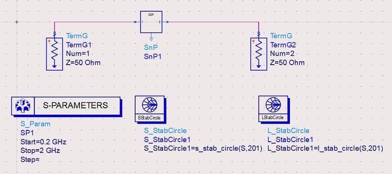
Figure 1. Input terminations, output terminations, and S-parameters in PathWave ADS.

 

The s2p component should be provided with an S-parameters file, which is most commonly in the Touchstone file format. The S-parameters data provided in Table 1 gives us the Touchstone file in Table 3. We save this as a text file with the .s2p extension and link it to the PathWave ADS s2p component.

 

Table 3. Touchstone S-parameter file.

 

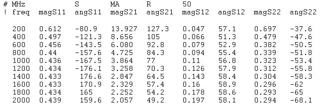
The options line, which starts with a # symbol, contains the header information. It specifies the frequency unit (Hz, KHz, MHz, or GHz) and the data format used. As in Table 1, the frequency unit here is MHz. With a Touchstone file, we have three data format options for entering the complex-valued S-parameters:

1. Magnitude/angle.
2. dB/angle.
3. Real/imaginary.

Table 3 provides the data in magnitude/angle format. This is specified by “MA” in the options line. To the right of “MA” on the same line, the term “R 50” indicates that the load termination resistor for the S-parameters is 50 Ω.

Comments in a Touchstone file start with the ! symbol. The comment line in Table 3 shows that the first column is frequency, the second column is magnitude of S₁₁, the third column is angle of S₁₁, and so on. Since we have the S-parameters at 10 frequency points, there are 10 rows of numbers in our file.

In the above schematic, the SStabCircle and LStabCircle functions allow us to plot the input and output stability circles, respectively. By running the simulation, we obtain the input stability circles plotted in Figure 2.

 

Figure 2. Input stability circles plotted in PathWave ADS using the data in Table 3.

 

Figure 3 shows the output stability circles.

 

Figure 3. Output stability circles plotted in PathWave ADS using the data in Table 3.

 

Finding the Stabilizing Parallel Resistor

By adding a parallel resistor to the input and/or output port of a potentially unstable transistor, we can create an unconditionally stable device. The added resistor throws away a portion of the power gain and leads to stable operation. However, we need to determine the appropriate value of the stabilizing resistor.

Consider the output stability circles we plotted in Figure 3. To find the appropriate value of the parallel resistor, we first need to find the constant conductance circle of the Smith chart that’s tangent to the most restrictive stability circle. This turns out to be the g = 0.6 constant conductance circle, which is marked in blue in Figure 4. Its point of intersection with the stability circle is labeled as “m1.”

 

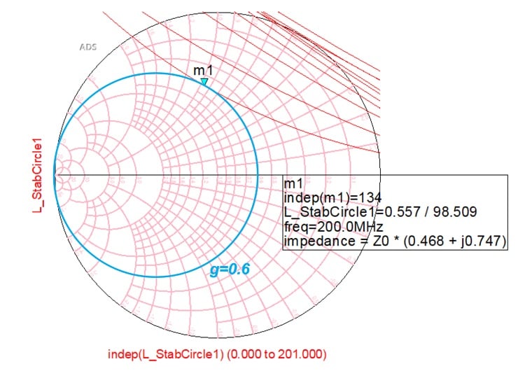
Figure 4. The g = 0.6 constant conductance circle (marked in blue). It intersects the most restrictive stability circle at point m1.

 

We can also calculate the conductance of this constant conductance circle by converting the impedance associated with the m1 marker to its equivalent admittance (y):

$$y~=~\frac{1}{0.468~+~j0.747}~=~0.6023~-~j0.9613$$

Equation 4.

 

With a reference impedance of 50 Ω, the g = 0.6 circle corresponds to a conductance of 12 mS or a resistance of 83.3 Ω. If we add this resistor in parallel with the output port, the overall load resistance seen by the output port is always less than 83.3 Ω.

Put another way, the overall normalized conductance seen by the output port is always greater than 12 mS. Γ_L is therefore always inside of the g = 0.6 circle and outside of the stability circles. Figure 5 shows the new schematic, which includes the stabilizing output resistor.

 

Figure 5. PathWave ADS schematic of a transistor with a stabilizing output resistor added.

 

You can use an RF simulator to verify that both input and output stability circles of the new circuit do not intersect the Smith chart. In the above schematic, the stability measurement equation “Mu” has been added to calculate the μ factor.

There are two μ factors for stability analysis in RF designs: μ₁ and μ₂. Equation 3 gives us μ₂. By swapping S₁₁ for S₂₂ in Equation 3, we obtain the equation for the μ₁ factor. Note that if either μ factor is greater than 1, so is the other. μ₁ is calculated in the schematic above—the results of these calculations are plotted in Figure 6.

 

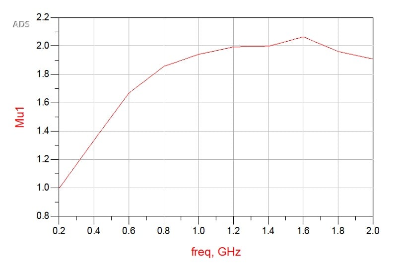
Figure 6. Plot of μ₁ vs. frequency for the transistor in Figure 5.

 

As you can see, by adding the stabilizing resistor, the circuit becomes unconditionally stable over the 0.2 GHz to 2 GHz frequency range. To create an added margin of stability, we can use a slightly lower value of parallel resistance to ensure that different non-idealities don’t move us to the unstable region.

Due to the coupling between the input and output ports, we usually need to stabilize only one of the ports. In the above example, we added the stabilizing resistor only to the output port, and this made the entire circuit unconditionally stable.

 

Finding the Stabilizing Series Resistor

Alternatively, we can add a series resistor (Figure 7) to the input and/or output port of a potentially unstable transistor to create an unconditionally stable device.

 

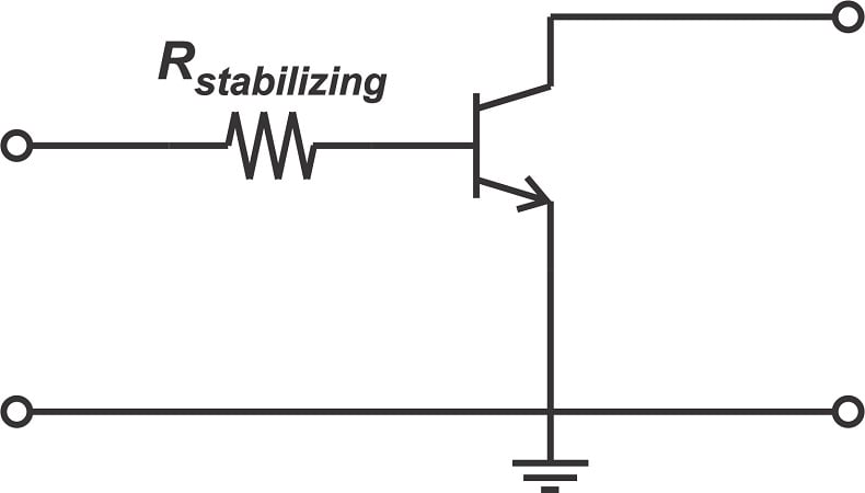
Figure 7. A stabilizing series resistor added to a transistor.

 

We need to find the constant resistance circle of the Smith chart that’s tangent to the most restrictive stability circle. We’re adding the resistor at the input port this time, so we’ll be considering the input stability circles in Figure 2. As Figure 8 shows, the r = 0.75 constant resistance circle is tangent to the most restrictive stability circle.

 

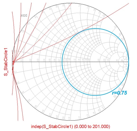
Figure 8. The r = 0.75 constant resistance circle (marked in blue) is tangent to the most restrictive stability circle.

 

With a reference impedance of 50 Ω, r = 0.75 corresponds to a resistance of 37.5 Ω. If we add this series resistor to the input of the device, we can ensure that the overall resistance seen by the device is always greater than or equal to 37.5 Ω. Therefore, Γ_S is always outside of the stability circles, and we have a stable operation. In order to have an added margin of safety, we usually use a slightly higher value of series resistance.

 

Wrap-Up

We examined two different tests for unconditional stability in this article, followed by two different ways to stabilize a potentially unstable device through resistive loading. We also introduced PathWave ADS, which we’ll use further in future articles. In short, we’ve covered a great deal of material—I hope you’ve found it both interesting and informative. Next time, we’ll begin discussing the design of low-noise amplifiers.

 

Featured image used courtesy of Adobe Stock; all other images used courtesy of Steve Arar