The Nyquist–Shannon Theorem: Understanding Sampled Systems

Modern technology as we know it would not exist without analog-to-digital conversion and digital-to-analog conversion. In fact, these operations have become so commonplace that it sounds like a truism to say that an analog signal can be converted to digital and back to analog without any significant loss of information.

But how do we know that this is indeed the case? Why is sampling a non-destructive operation, when it appears to discard so much signal behavior that we observe between the individual samples?

How on earth can we start with a signal that looks like this:

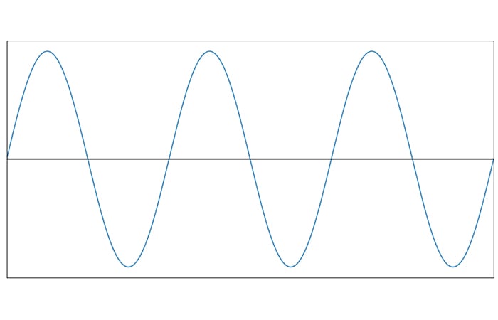
And digitize it into this:

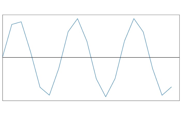
And then dare to claim that the original signal can be restored with no loss of information?

The Nyquist–Shannon Theorem

Such a claim is possible because it is consistent with one of the most important principles of modern electrical engineering:

If a system uniformly samples an analog signal at a rate that exceeds the signal’s highest frequency by at least a factor of two, the original analog signal can be perfectly recovered from the discrete values produced by sampling.

There is much more that needs to be said about this theorem, but first, let’s try to figure out what to call it.

Shannon? Nyquist? Kotelnikov? Whittaker?

I am certainly not the person to decide who deserves the most credit for formulating, demonstrating, or explaining the Shannon–Nyquist–Kotelnikov–Whittaker Theory of Sampling and Interpolation. All four of these individuals had some sort of prominent involvement.

However, it does appear that the role of Harry Nyquist has been extended beyond its original significance. For example, in Digital Signal Processing: Fundamentals and Applications by Tan and Jiang, the principle stated above is identified as the “Shannon sampling theorem,” and in Microelectronic Circuits by Sedra and Smith, I find the following sentence: “The fact that we can do our processing on a limited number of samples … while ignoring the analog-signal details between samples is based on … Shannon’s sampling theorem.”

Thus, we probably should avoid using “the Nyquist sampling theorem” or “Nyquist’s sampling theory.” If we need to associate a name with this concept, I suggest that we include only Shannon or both Nyquist and Shannon. And in fact, maybe it’s time to transition to something more anonymous, such as “Fundamental Sampling Theorem.”

If you find this somewhat disorienting, remember that the sampling theorem stated above is distinct from the Nyquist rate, which will be explained later in the article. I don’t think that anyone is trying to separate Nyquist from his rate, so we end up with a good compromise: Shannon gets the theorem, and Nyquist gets the rate.

Sampling Theory in the Time Domain

If we apply the sampling theorem to a sinusoid of frequency f_SIGNAL, we must sample the waveform at f_SAMPLE ≥ 2f_SIGNAL if we want to enable perfect reconstruction. Another way to say this is that we need at least two samples per sinusoid cycle. Let’s first try to understand this requirement by thinking in the time domain.

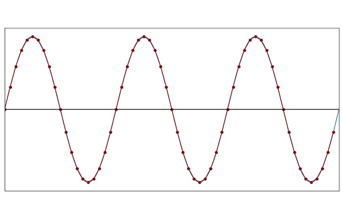
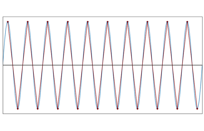
In the following plot, the sinusoid is sampled at a frequency that is much higher than the signal frequency.

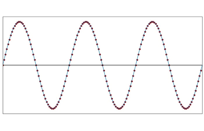
Each circle represents a sampling instant, i.e., a precise moment at which the analog voltage is measured and converted into a number.

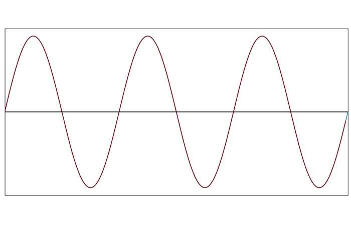
To better visualize what this sampling procedure has given us, we can plot the sample values and then connect them with straight lines. The straight-line approximation shown in the next plot looks exactly like the original signal: the sampling frequency is very high relative to the signal frequency, and consequently the line segments are not noticeably different from the corresponding curved sinusoid segments.

As we reduce the sampling frequency, the appearance of the straight-line approximation diverges from the original.

20 samples per cycle (f_SAMPLE = 20f_SIGNAL)

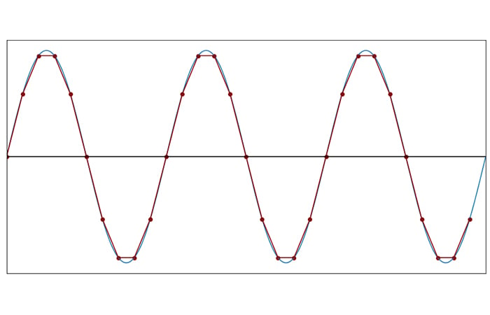
10 samples per cycle (f_SAMPLE = 10f_SIGNAL)

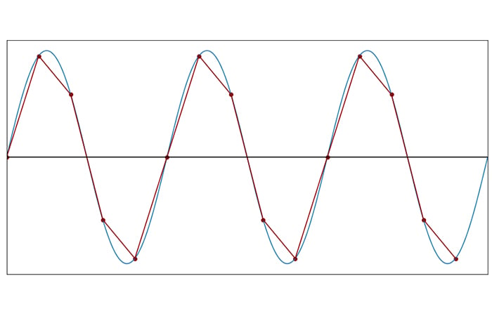
5 samples per cycle (f_SAMPLE = 5f_SIGNAL)

At f_SAMPLE = 5f_SIGNAL, the discrete-time waveform is no longer a pleasing representation of the continuous-time waveform. However, notice that we can still clearly identify the frequency of the discrete-time waveform. The cyclic nature of the signal has not been lost.

The Threshold: Two Samples per Cycle

The data points produced by sampling will continue to retain the cyclic nature of the analog signal as we decrease the number of samples per cycle below five. However, eventually we reach a point at which frequency information is corrupted. Consider the following plot:

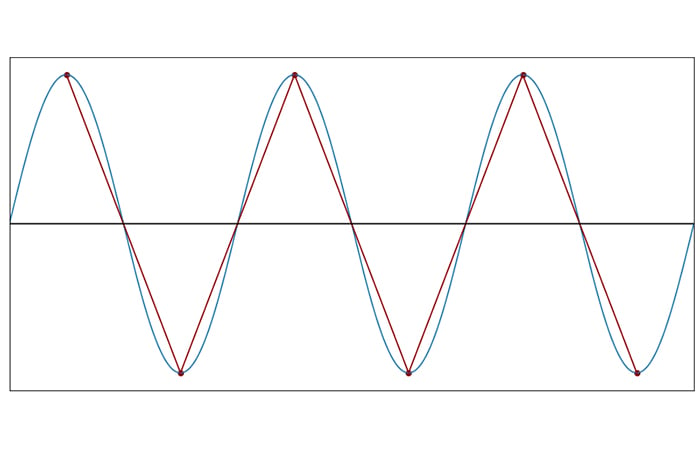
2 samples per cycle (f_SAMPLE = 2f_SIGNAL)

With f_SAMPLE = 2f_SIGNAL, the sinusoidal shape is completely gone. Nevertheless, the triangle wave created by the sampled data points has not altered the fundamental cyclical nature of the sinusoid. The frequency of the triangle wave is identical to the frequency of the original signal.

However, as soon as we reduce the sampling frequency to the point at which there are fewer than two samples per cycle, this statement can no longer be made. Two samples per cycle, for the highest frequency in the original waveform, is therefore a critically important threshold in mixed-signal systems, and the corresponding sampling frequency is called the Nyquist rate:

If we sample an analog signal at a frequency that is lower than the Nyquist rate, we will not be able to perfectly reconstruct the original signal.  

The next two plots demonstrate the loss of cyclical equivalency that occurs when the sampling frequency drops below the Nyquist rate.

2 samples per cycle (f_SAMPLE = 2f_SIGNAL)

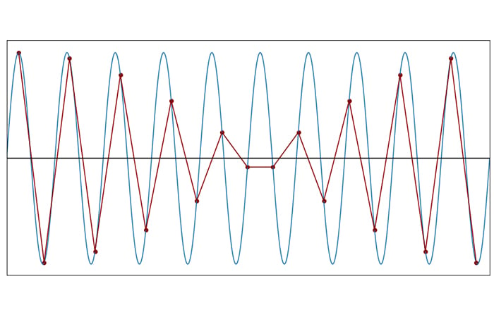
1.9 samples per cycle (f_SAMPLE = 1.9f_SIGNAL)

At f_SAMPLE = 1.9f_SIGNAL, the discrete-time waveform has acquired fundamentally new cyclical behavior. Full repetition of the sampled pattern requires more than one sinusoid cycle.

However, the effect of insufficient sampling frequency is somewhat difficult to interpret when we have 1.9 samples per cycle. The next plot makes the situation more clear.

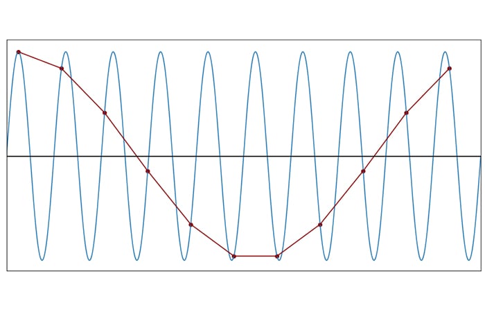
1.1 samples per cycle (f_SAMPLE = 1.1f_SIGNAL)

If you knew nothing about a sinusoid and performed an analysis using the discrete-time waveform resulting from sampling at 1.1f_SIGNAL, you would form seriously erroneous ideas about the frequency of the original signal. Furthermore, if all you have is the discrete data, it is impossible to know that frequency characteristics have been corrupted. Sampling has created a new frequency that was not present in the original signal, but you don’t know that this frequency was not present.

The bottom line is this: When we sample at frequencies below the Nyquist rate, information is permanently lost, and the original signal cannot be perfectly reconstructed.

Conclusion

We’ve covered the Shannon sampling theorem and the Nyquist rate, and we tried to gain some insight into these concepts by looking at the effect of sampling in the time domain. In the next article, we’ll explore this topic from the perspective of the frequency domain.