Multirate DSP and Its Application in D/A Conversion

This article reviews the basics of D/A conversion and explains how multirate DSP can lead to a more efficient system.

In part one of this series, you can read about this topic for A/D conversion: Multirate DSP and Its Application in A/D Conversion.

The Conceptual Operation of an Ideal DAC

As shown in Figure 1, an ideal D/A converter receives a sequence of quantized values, $$y(n)$$, and generates a weighted impulse train, $$y_{s}(t)$$. As the graph of $$y(n)$$ in Figure 1 implies, $$y(n)$$ is a discrete sequence of values. We know the value of $$y(n)$$ for a specific $$n$$, but the graph does not provide any information about the sampling rate with which the underlying continuous-time signal was sampled. The D/A stage needs to know the sampling period, $$T$$, to produce the impulse corresponding to a particular value of $$y(n)$$ at the time $$nT$$.

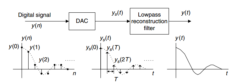
Figure 1. The operation of an ideal D/A converter. Image courtesy of Digital Signal Processing.

Suppose that each value of $$y(n)$$ is represented by $$m$$ bits, $$y_{m-1}y_{m-2} \dots y_{0}$$, and the converter is a binary-weighted one. Hence, we have

$$y_{s}(nT)= \sum_{k=0}^{m-1}y_{k}2^{k}R_{ref}$$

where $$R_{ref}$$ is a reference voltage, current, or charge. So far, our ideal D/A stage has converted a discrete-time quantized sequence, $$y(n)$$, into a continuous-time analog signal, $$y_{s}(t)$$.

Why Do We Need a Reconstruction Filter after a DAC?

$$y_{s}(t)$$ is equal to the underlying continuous-time signal, $$y_{c}(t)$$, only at $$t=nT$$, and it is zero otherwise. How can we recover the original $$y_{c}(t)$$ from $$y_{s}(t)$$? Assume that $$y(n)$$ was obtained by sampling the original signal, $$y_{c}(t)$$, with a sampling period of $$T$$. Hence,

$$y_{s}(t)=y_{c}(t) \times \sum_{n=- \infty}^{+ \infty} \delta(t-nT)$$

In a previous article, we saw how multiplying a continuous-time signal, $$y_c(t)$$, by an impulse train with period $$T$$ leads to replicas of the spectrum of $$y_c(t)$$ at multiples of $$\frac{2\pi}{T}$$. That’s why $$y_s(t)$$ in Figure 1 contains not only the spectrum of the underlying continuous-time signal but also its replicas at multiples of the sampling frequency. This is illustrated in Figure 2. To recover $$y_c(t)$$, we need to get rid of the high-frequency components. This is achieved by the analog lowpass filter of Figure 1, which is called a reconstruction filter.

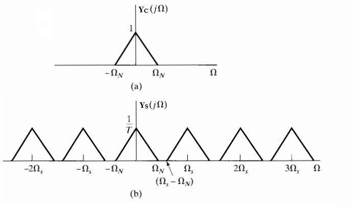
Figure 2. Multiplying a signal by an impulse train leads to replicas of the input spectrum at multiples of the sampling frequency $$\Omega_s$$. Image courtesy of Discrete-Time Signal Processing.

To further clarify the requirements of the reconstruction filter, assume that we have utilized a sampling frequency of $$2 \Omega_N$$ to sample $$y_c(t)$$, which has all its energy below $$\Omega_N$$, i.e., $$Y_c(j\Omega)=0$$ for $$| \Omega | > \Omega_N$$. In this case, we need a sharp reconstruction filter which passes the frequency components up to $$\Omega_N$$ and eliminates the unwanted frequency components of $$Y_s(j\Omega)$$ just above $$\Omega_N$$. Since this sharp filtering characteristic is not practical, we need to change our design.

For a given $$Y_c(j\Omega)$$, if we increase the sampling frequency, the replicas would go to higher frequencies, and the reconstruction filter could have a smoother transition from passband to stopband. For example, assume that $$y_c(t)$$ represents an analog music waveform with energy in the band $$0< \frac{|\Omega|}{2 \pi} < 22 kHz$$. If we had sampled $$y_c(t)$$ with a sampling frequency $$8$$ times higher than the Nyquist sampling rate, $$f_{s, new}=352 kHz$$, then the reconstruction filter would have had a transition band of $$(\Omega_s - \Omega_N)- \Omega_N=2 \pi \times 308 kHz$$ (see Figure 2). However, it is not efficient to use $$352,000$$ samples per second to represent a signal which has all its energy below $$22 kHz$$. For example, this sampling scheme would increase the memory for storing the samples by $$8$$ times compared to a system which uses $$f_s=44 kHz$$. That’s why, even if we have utilized oversampling during A/D conversion, we apply decimation to our digital data to reduce the number of samples.

As a result, $$y(n)$$ will generally use the smallest possible number of samples to represent a given $$y_c(t)$$. The question is: can we process y(n) in the digital domain and increase the sample rate by interpolating between the existing samples? If we can do this, we can increase the sample rate and thereby achieve the important goal of relaxing the requirements of the reconstruction filter.

Interpolation

We want to digitally increase the sampling rate of $$y(n)$$, but how? Suppose that we place $$L-1$$ zero-valued samples between adjacent samples of $$y(n)$$ (see Figure 3 for $$L=2$$).

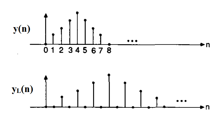
Figure 3. Adding one zero-valued sample between adjacent samples of a discrete-time signal. Image courtesy of IEEE.

Obviously, this increases the sample rate, but the samples that we have added essentially seem to carry no information, because they are not at all related to the existing samples of $$y(n)$$. However, examining the Fourier transform of the obtained sequence proves to be worthy. Let’s name the new sequence $$y_l(n)$$, then we have $$y_l(n)=y(n\text{/}L)$$ when $$n$$ is a multiple of $$L$$ and zero otherwise. We obtain the Fourier transform of $$y_l(n)$$ as

$$Y_l(e^{j\omega})=\sum_{n=- \infty}^{+\infty}y_l(n)e^{-jn\omega}$$

However, $$y_l(n)$$ is non-zero only when $$n=kL$$, where $$k$$ is an integer. Considering the fact that non-zero values of $$y_l(n)$$ are related to $$y(n)$$, we obtain

$$Y_l(e^{j\omega})=\sum_{k=-\infty}^{+\infty}y_l(kL)e^{-jkL\omega}=\sum_{k=-\infty}^{+\infty}y(k)e^{-jkL\omega}=Y(e^{jL\omega})$$

The above equation means that the spectrum of $$y_l(n)$$ is the same as that of $$y(n)$$ except for scaling which needs to be applied to the $$\omega$$ axis. This is illustrated in Figure 4.

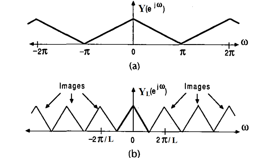
Figure 4. The effect of adding L-1 zero-valued samples between adjacent samples of y(n). Image courtesy of IEEE.

Examining the above spectra, we see that it is possible to extract the spectrum of $$Y(e^{j\omega})$$ from that of $$Y_l(e^{j\omega})$$. To this end, we only need to apply a sharp low-pass filter with the normalized cutoff frequency of $$\frac{\pi}{L}$$ to $$y_l(n)$$. This will omit all the frequency components above $$\frac{\pi}{L}$$, which are generally referred to as images (see Figure 4). Note that this filter is digital, and we can achieve a sharp magnitude response along with a linear phase response in the digital domain.

While Figure 4 suggests that the $$\omega$$ axis of $$Y_l(e^{j\omega})$$ is scaled compared to the spectrum of $$Y(e^{j\omega})$$, there is no frequency scaling if we consider the frequency in terms of cycles per second. We know that $$f=\frac{\omega}{2\pi T}$$, where $$T$$ is the sampling period and $$\omega$$ is the normalized frequency. In Figure 4(a), the sampling period is $$T=\frac{1}{f_s}$$, and the point associated with $$\omega=\pi$$ gives $$f=\frac{f_s}{2}$$. In Figure 4(b), the sampling period is $$\frac{T}{L}$$ and $$\omega=\frac{\pi}{L}$$ corresponds to

$$f=\frac{ \frac{\pi}{L} } { 2\pi \frac{T}{L} }= \frac{f_s}{2}$$   

Therefore, while the sample rate is increased by $$L$$, there is no scaling on the frequency axis if we consider the frequency in terms of cycles per second.

In summary, to increase the sampling rate of a discrete-time sequence $$y(n)$$, we place $$L-1$$ zero-valued samples between adjacent samples and apply a lowpass filter with the normalized cutoff frequency of $$\frac{\pi}{L}$$ to the obtained sequence. This is illustrated in Figure 5.

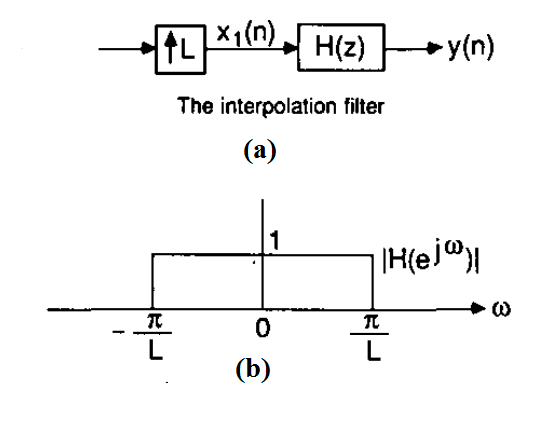
Figure 5. Upsampling followed by a low-pass filter with a normalized cutoff frequency of $$\frac{\pi}{L}$$ performs interpolation. Image courtesy of IEEE.

Now, let’s go back to the problem of designing an efficient D/A stage.

Interpolation Relaxes the Requirements of the Reconstruction Filter

As discussed above, increasing the sampling rate of $$y(n)$$ can move replicas of the spectrum of $$y_c(t)$$ to higher frequencies and thereby make the implementation of the analog filter more feasible. Figure 6 shows how we can apply interpolation in the digital domain before the D/A stage.

Figure 6. Interpolation prior to the D/A stage. Image courtesy of Digital Signal Processing.

As shown in the figure, there are two sample rates in this system, $$f_s$$ and $$Lf_s$$. The interpolation filter has a cutoff frequency of $$\frac{fs}{2}$$ and is used to remove the images discussed above. In this way, the requirements for the analog filter are less demanding because it only needs to suppress the very-high-frequency components that are at multiples of $$Lf_s$$.

Zero-Order Hold at the Output of a Practical D/A Converter

In Figure 1, we assumed that the output of an ideal DAC is an impulse train; however, in practice, it is not possible to generate these narrow pulses. Instead, a practical DAC generally holds the last output value until the next value is generated. This is called zero-order hold and can be represented by placing a sample-and-hold at the output of an ideal DAC (see Figure 7).

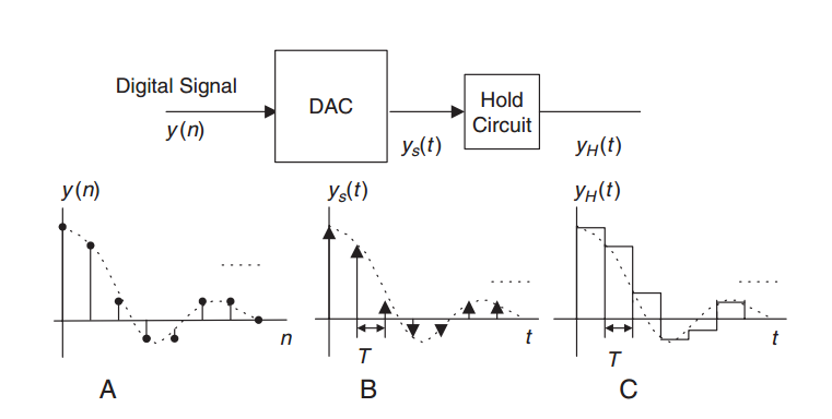
Figure 7. Practical DACs generally apply zero-order hold to the output values. Image courtesy of Digital Signal Processing.

As the figure suggests, the spectrum of $$y_s(t)$$ must be multiplied by the transfer function of the zero-order hold block. It can be shown that the transfer function of zero-order hold is

$$H(j\Omega)=t_h \frac{sin( \Omega \frac{t_h}{2})} { \Omega \frac{t_h}{2}}$$

Equation 1

where $$t_h$$ denotes the hold time, which is generally equal to the sampling period, $$T=\frac{1}{f_s}$$.

Assume that $$y(n)$$ in Figure 7 corresponds to a continuous-time signal $$y_c(t)$$ that has all its energy below $$f_N=\frac{f_s}{2}$$, and that we have obtained $$y(n)$$ by sampling $$y_c(t)$$ with sampling rate $$f_s$$. In this case the response of the zero-order hold and the spectrum of $$y_s(t)$$ will be as shown in Figure 8.

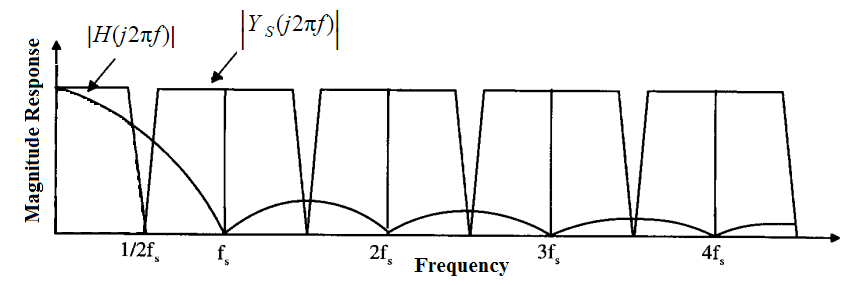
Figure 8. The magnitude response of the zero-order hold, $$H(j2 \pi f)$$, and the spectrum of $$y_s(t)$$. Image courtesy of CMOS Integrated Analog-to-Digital and Digital-to-Analog Converters.

Figure 8 shows that the frequency components of $$y_c(t)$$ that are around $$\frac{f_s}{2}$$ are attenuated much more than the low-frequency components. Examining $$H(j\Omega)$$ at $$\Omega=0$$ and $$\Omega=2 \pi \frac{f_s}{2}$$, we observe that the zero-order hold function exhibits nearly $$3.9 dB$$ more attenuation for $$\Omega=2 \pi \frac{f_s}{2}$$ than for the low-frequency components near $$\Omega=0$$. This is a well-known amplitude reduction called $$\frac{sin(x)}{x}$$ distortion.

Now, suppose that we apply L-fold interpolation to $$y(n)$$ and increase the sample rate to $$f_{s, new}=Lf_s$$. In this case, we have $$t_h=\frac{1}{Lf_s}$$. What would be the attenuation of $$H(j\Omega)$$ for the high-frequency components of $$y_c(t)$$ around $$f_N=\frac{f_s}{2}$$? Substituting the values in Equation 1, we obtain

$$| H(j0) |=t_h$$

$$| H(j2\pi \frac{f_s}{2}) | =t_h \frac{ sin( \frac{\pi}{2L} ) } { \frac{\pi}{2L}}$$

As we use a larger $$L$$, $$\frac{sin( \frac{\pi}{2L} ) } { \frac{\pi}{2L} }$$ tends toward one and the attenuation of $$H(j\Omega)$$ decreases.

In summary, interpolation not only relaxes the requirements of the reconstruction filter but also makes the $$\frac{sin(x)}{x}$$ distortion less severe.

Summary

• An ideal D/A converter receives a sequence of quantized values, $$y(n)$$, and generates a weighted impulse train, $$y_s(t)$$.
• $$y_s(t)$$ contains not only the spectrum of the underlying continuous-time signal but also its replicas at multiples of the sampling frequency.
• To recover $$y_c(t)$$, we need to remove the high-frequency components using a reconstruction filter.
• For a given $$Yc(j\Omega)$$, if we increase the sampling frequency, the replicas would go to higher frequencies, and the reconstruction filter could have a smoother transition from passband to stopband.
• To increase the sampling rate of a discrete-time sequence, $$y(n)$$, we place $$L-1$$ zero-valued samples between adjacent samples and apply a low-pass filter with normalized cutoff frequency of $$\frac{\pi}{L}$$ to the obtained sequence.
• In this way, the requirements for the analog filter become much less demanding because it only needs to suppress some very-high-frequency components.
• Interpolation not only relaxes the requirements of the reconstruction filter but also makes the $$\frac{sin(x)}{x}$$ distortion less severe.

For a more detailed discussion on $$\frac{sin(x)}{x}$$ distortion and a review of methods of reducing it, see CMOS Integrated Analog-to-Digital and Digital-to-Analog Converters and Discrete-Time Signal Processing.

• Next Article →