LVDT Demodulation: Rectifier-Type vs. Synchronous Demodulation

In a previous article, we discussed the operation and challenges of a diode rectifier demodulator. In this article, we’ll first look at the limitations of the rectifier type demodulators in general. Then, we’ll see that a synchronous demodulator can address some of these problems. Finally, we’ll look at the disadvantages of synchronous demodulation in LVDT applications. 

 

Limitations of Rectifier Type Demodulators

Although a precision rectifier can remedy the challenges of a simple diode rectifier, rectifier type demodulators have several downsides in general. With a rectifier-type demodulator, we need access to the center tap of the LVDT secondary to rectify the voltage across each of the secondary windings. Therefore, this type of demodulation is only applicable to 5-wire LVDTs (Figure 1(b)).

 

Figure 1. (a) 4-wire and (b) 5-wire LVDTs.

 

There are other demodulation methods that don’t need access to the center tap and can determine the core position by processing the voltage difference between the two secondaries. These demodulators allow us to employ a 4-wire LVDT as depicted in Figure 1(a). 

Is it really important to have the minimum number of electrical connections?

There are many applications where the conditioning circuitry is located at a long distance from the sensor. A good example is making measurements in harsh environments of radioactive applications where the conditioning circuitry should be placed in safe areas, even up to several hundred meters away from the LVDT. In these cases, it can be challenging to transmit the two secondary voltages over a long distance through a 5-wire configuration. With the conditioning module located away from the LVDT, it is necessary to have a well-balanced wiring with low distributed capacitance. This means a considerable increase in the cost of wiring.

Another disadvantage of a rectifier-type demodulator is its limited noise rejection. Consider an LVDT sensor with the core displacement following a sinusoidal waveform at 250 Hz. The red curve in Figure 2 shows the demodulated output of this LVDT obtained using a typical diode rectifier.

 

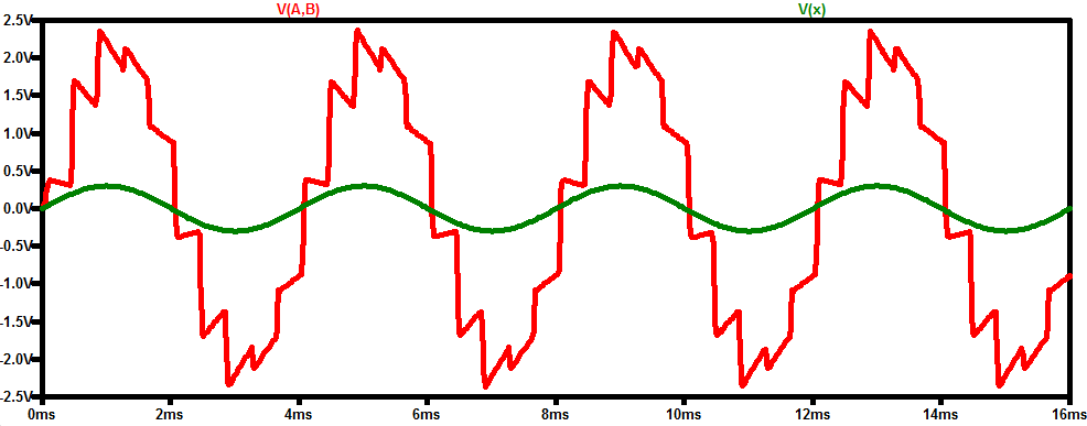
Figure 2.

 

In this figure, the green curve shows the core displacement x. As you can see, the output signal looks like the amplified version of x except that it has some abrupt changes corresponding to some high-frequency components.

To get rid of these unwanted high-frequency components, we can use a low-pass filter with a cutoff frequency slightly higher than the mechanical bandwidth of the system (250 Hz). Therefore, even with an ideal low-pass filter, all the frequency components up to 250 Hz will pass the filter without being attenuated. Hence, any noise component below 250 Hz that couples to the sensor output will appear at the demodulator output as well.

Poor noise performance is a major drawback of the rectifier type demodulators. This limitation becomes even more pronounced with long cables. The noise performance along with the 5-wire configuration requirement make this circuit unsuitable for long cable runs to remote locations. Synchronous demodulation discussed below can address these two problems. 

 

Synchronous Demodulation

Consider the LVDT shown in Figure 3. Assume that we have \[V_{EXC} = A_p\cos(2\pi \times f_p \times t)\].

 

Figure 3. An example LVDT

 

The differential output (\[V_{out}\]) is an amplitude modulated signal and can be expressed as:

 

\[V_{out} = A_s \times x \times \cos(2\pi \times f_p \times t + \phi)\]

Equation 1.

 

where x is the core displacement and \[A_s\] is a scaling factor that gives the overall output amplitude for a given x. The phase term \[\phi\] is the phase difference caused by the LVDT between the primary and secondary voltages. This phase shift should be ideally very small, especially around a specific frequency given by the manufacturer. However, we usually need to take this phase shift into account. 

The synchronous demodulation technique multiplies the LVDT differential output by the excitation signal (or a signal synchronous with the excitation signal in general). This gives:

 

\[V_{demod} = V_{out} \times V_{EXC} = A_s \times x \times \cos(2\pi \times f_p \times t + \phi) \times A_p\cos(2\pi \times f_p \times t)\]

Equation 2.

 

that simplifies to:

 

\[V_{demod} = \frac{1}{2} \times A_s \times x \times A_p [\cos(\phi) + \cos(2\pi \times 2f_p \times t + \phi)]\]

 

The first term inside the brackets is DC, however, the second term is at twice the excitation frequency. Hence, a narrow low-pass filter can remove the second term and we have:

 

\[V_{filtered} = \frac{1}{2} \times A_s \times x \times A_p\cos(\phi)\]

Equation 3.

 

This gives us a DC voltage proportional to the core displacement x.

 

Synchronous Demodulation Through Multiplying by a Square Wave

We can use an analog multiplier to multiply the LVDT output by the excitation sine wave (Equation 2); however, analog multipliers are expensive and have linearity limitations. Instead of multiplying by a sine wave, we can multiply the signal by a square wave synchronous with the excitation input. 

You might wonder how can a square wave be used instead of a sinusoidal? A square wave toggling between ±1 can be expressed as an infinite sum of sinusoids at the odd harmonics of the square wave frequency. Hence, a square wave of frequency \[f_p\] can be expressed as:

 

\[v_{squarewave}(t) = \sum_{n=1, 3, 5}^{\infty}\frac{4}{n\pi}\sin(2\pi \times nf_p \times t)\]

 

When the LVDT output (a sinusoidal at \[f_p\]) is multiplied by the square wave, the fundamental component of the square wave \[(\frac{4}{\pi}\sin(2\pi \times f_p \times t))\] produces a DC component as well as a high-frequency component at \[2f_p\]. The high-frequency component will be suppressed by a low-pass filter as explained in the previous section and the DC component which is the desired one will appear at the output.

Multiplication by the higher-order harmonics of the square wave will produce high-frequency components at even multiples of \[f_p\]. Hence, the DC component is the only one that appears at the filter output just as in the case of multiplying the signal by a sinusoidal. The main advantage of multiplying by a square wave is that it can significantly simplify the circuit implementation of the demodulator.

 

Circuit Implementation of a Synchronous Demodulator

The square wave-based synchronous demodulator is shown in Figure 4.

 

Figure 4. A square wave-based synchronous demodulator

 

In this case, the amplified version of the LVDT output is multiplied by a square wave rather than the excitation sinusoidal. The square wave is synchronous with the excitation input and is obtained through a “Zero-Crossing Detector” as shown in the above block diagram.

In order to perform multiplication by a square wave, the gain of the signal chain is periodically changed between \[±A_{amp}\] (\[A_{amp}\] is the amplifier gain). Note that the lower path incorporates a gain of -1. This is achieved by using the square wave to drive the switch SW that changes the signal path between the upper and the lower path. This is effectively equivalent to multiplying the amplifier output by the square wave.

Finally, a low-pass filter is used to keep the DC term of the output and suppress the high-frequency components.

 

The Pros of the LVDT Synchronous Demodulators

The main advantage of synchronous demodulation is its noise performance. As discussed above, synchronous demodulation frequency shifts the LVDT output to DC and uses a low-pass filter to keep this DC component. The low-pass filter will suppress all noise components outside of its passband.

Since our desired signal is at DC, we can use a narrow low-pass filter. This will limit the system bandwidth and allow the demodulator to significantly suppress a large portion of the noise that couples to the LVDT output. Moreover, with synchronous demodulation, we can use a 4-wire LVDT.

 

The Cons of the LVDT Synchronous Demodulators

Although synchronous demodulation can offer a higher noise immunity compared to the rectifier type demodulators, its output depends on the amplitude of the excitation voltage (\[A_p\] in Equation 3). Hence, with synchronous demodulation, the amplitude stability of the excitation input is critical.

Another issue is that the demodulator output depends on the phase shift of the LVDT transfer function (\[\cos(\phi)\] in Equation 3). This phase shift should be ideally very small; however, it is not constant and can change with the operating point. Practical demodulator circuits commonly employ a phase compensation network to adjust the phase of the produced square wave. The compensation network can increase the complexity of the demodulator.

However, this increased complexity makes the circuit suitable for relatively longer cables when compared with the rectifier-type demodulators. This is due to the fact that the phase shift term \[\phi\] can be used to take the delay caused by the wiring into account. Hence, the phase compensation circuitry can also be used to compensate for the cable delay and make the circuit suitable for longer wires.

 

Other Demodulation Techniques

Synchronous demodulation offers a higher noise immunity and requires only four electrical connections; however, it has its own limitations such as dependence on the amplitude of the excitation input as well as the phase shift issue. To address these problems, there are several other demodulation techniques. These techniques usually employ ratiometric measurement concepts and DSP-based methods to circumvent the limitation of synchronous demodulators. 

For a more detailed discussion of synchronous demodulation when applied to other sensor types, please refer to the following articles:

• Introduction to the Synchronous Demodulation
• Synchronous Demodulation Using Analog Multipliers vs. Switch-based Multipliers
• Analog and Digital Implementation of a Synchronous Demodulator

To see a complete list of my articles, please visit this page.