Unconditional Stability and Potential Instability in RF Amplifier Design

If you’re designing an active RF circuit, you should always start with a thorough stability analysis. In this article, we’ll learn about basic concepts related to stability analysis, including input and output stability circles. We’ll also learn how the arrangement of these circles on a Smith chart can produce either unconditionally stable or potentially unstable devices.

First, though, why is stability analysis so important?

 

Why We Need Stability Analysis

At high frequencies, unavoidable parasitic effects can easily make the circuit oscillate. For example, a poor grounding scheme can cause coupling between different stages of a multi-stage amplifier and lead to instability.

Also, some circuits in the RF signal chain might not have a well-defined source or load impedance. For example, the low noise amplifier (LNA) in a receiver needs to interface with the outside world through the antenna. The impedance of the antenna can change if the user brings their hand close to the antenna, so the LNA must remain stable for all possible values of the source impedance at all frequencies.

Sometimes instability can have strange indications, like abrupt changes in the DC parameters of the amplifier, or high sensitivity of the circuit to its surroundings. This can make conducting a properly thorough stability analysis a challenging, intricate task.

 

Single-Stage RF Amplifier

Figure 1 shows the basic layout of an RF amplifier.

 

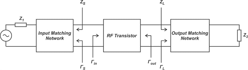
Figure 1. Diagram of a basic single-stage RF amplifier.

 

In the diagram above, matching networks are used on both sides of the transistor to transform input impedance (Z₁) and output impedance (Z₂) to the desired values Z_S and Z_L. The subscripts S and L denote, respectively, source and load.

In order to examine the circuit’s stability, we’ll model the active device as a two-port network (Figure 2). This two-port network will be characterized through its S-parameters and connected to impedances presented by the input and output matching networks Z_S and Z_L.

 

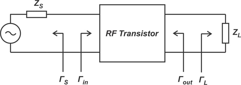
Figure 2. The circuit used to analyze the stability of an RF amplifier.

 

Using signal flow graph analysis, we can derive expressions for the reflection coefficients, Γ_IN and Γ_OUT, in terms of the transistor’s S-parameters:

$$\Gamma_{IN}~=~S_{11} + \frac{S_{12}S_{21} \Gamma_L}{1~-~S_{22}\Gamma_L}$$

Equation 1.

 

$$\Gamma_{OUT}~=~S_{22} + \frac{S_{12}S_{21} \Gamma_S}{1~-~S_{11}\Gamma_S}$$

Equation 2.

 

The above equations allow us to examine the stability of a two-port network. Remember that the magnitude of Γ is bounded between 0 and 1 for passive circuits. The reflected signal is therefore smaller than the incident signal. For an active device, however, the reflected signal can experience a gain rather than an attenuation.

In other words, for certain values of the S-parameters, the magnitude of the input and output reflection coefficients of an active device can be greater than unity (|Γ_IN| > 1 and/or |Γ_OUT| > 1). This can happen even though the source and load terminations of the transistor are passive (|Γ_S| < 1 and |Γ_L| < 1). Also, note that a reflection coefficient greater than unity corresponds to an impedance with negative real part. Oscillation is possible when either the input or output port produces a negative resistance.

 

Unconditional Stability and Potential Instability

A two-port network is said to be unconditionally stable if it can be connected to any source and load impedances without oscillations. In this context, we’re commonly referring to any passive source and load impedances—in other words, it’s assumed that |Γ_S| < 1 and |Γ_L| < 1. Thus, for an unconditionally stable transistor, the locus of the input and output reflection coefficients is the entire region inside of the Smith chart’s unit circle.

A transistor that is not unconditionally stable is usually described as a “potentially unstable” device. A potentially unstable device can become unstable for certain values of passive source and load impedances. Note that stability is frequency-dependent: a transistor might be unconditionally stable at a certain frequency range, but potentially unstable at a different frequency range. For that reason, the stability should be assessed at every frequency point where the transistor’s data is available.

In mathematical language, unconditional stability requires |Γ_IN| < 1 and |Γ_OUT| < 1. Therefore, we have:

$$|\Gamma_{IN}|~=~|S_{11} + \frac{S_{12}S_{21} \Gamma_L}{1~-~S_{22}\Gamma_L}|~<~1$$

Equation 3.

 

$$|\Gamma_{OUT}|~=~|S_{22} + \frac{S_{12}S_{21} \Gamma_S}{1~-~S_{11}\Gamma_S}~|~<1$$

Equation 4.

 

When the above conditions are satisfied, the real part of the impedance of the transistor’s input and output ports are positive for all passive source and load terminations. If these conditions are not met at a certain frequency, the transistor is potentially unstable at that frequency.

 

Input and Output Stability Circles

If we set |Γ_IN| and |Γ_OUT| equal to unity, we obtain equations that specify the boundary of instability:

$$|\Gamma_{IN}|~=~|S_{11} + \frac{S_{12}S_{21} \Gamma_L}{1~-~S_{22}\Gamma_L}|~=~1$$

Equation 5.

 

$$|\Gamma_{OUT}|~=~|S_{22} + \frac{S_{12}S_{21} \Gamma_S}{1~-~S_{11}\Gamma_S}|~=~1$$

Equation 6.

 

Equation 5 specifies all load reflection coefficients (Γ_L) that make the magnitude of the input reflection coefficient equal to 1 (|Γ_IN| = 1). Because this equation specifies the boundary for usable Γ_L values, it should be plotted in the Γ_L plane. By the same token, Equation 6 specifies the usable values of Γ_S, so it should be plotted in the Γ_S plane.

In their current forms, these equations are simple to interpret but difficult to work with. Fortunately, a bit of mathematical manipulation allows both equations to be put into the standard form for a circle equation. Equation 5 becomes:

$$|\Gamma_{L}~-~c_{L}|~=~r_L$$

Equation 7.

where c_L denotes the center of the circle and r_L denotes the circle’s radius.

To find c_L, we use Equation 8:

$$c_L~=~\frac{ \big ( S_{22}~-~\Delta S_{11}^* \big )^*}{|S_{22}|^2~-~|\Delta|^2}$$

Equation 8.

 

Equation 9 gives us r_L:

$$r_L~=~\Big | \frac{ S_{12} S_{21}}{|S_{22}|^2~-~|\Delta|^2} \Big |$$

Equation 9.

 

In the above equations, Δ is the determinant of the S-parameter matrix. It can be expressed as follows:

$$\Delta~=~S_{11}S_{22}~-~S_{12}S_{21}$$

Equation 10.

 

Since Equation 7 defines a circle that specifies the boundary for usable Γ_L values, we refer to the above circle as the output stability circle.

Similarly, Equation 6 corresponds to a circle centered at c_S:

$$c_S~=~\frac{ \big ( S_{11}~-~\Delta S_{22}^* \big )^*}{|S_{11}|^2~-~|\Delta|^2}$$

Equation 11.

and having radius r_S:

$$r_S~=~\Big | \frac{ S_{12} S_{21}}{|S_{11}|^2~-~|\Delta|^2} \Big |$$

Equation 12.

 

Because it specifies the usable Γ_S values, we call the circle produced by Equation 6 the input stability circle.

 

Example: Finding the Stability Circles

Table 1 gives the S-parameters for the Onsemi 2SC5226A NPN transistor at V_CE = 5 V and I_C = 7 mA.

 

Table 1. S-parameters for the 2SC5226A NPN transistor. Data used courtesy of Onsemi

Freq (MHz)	|S11|	∠ S11	|S21|	∠ S21	|S12|	∠ S12	|S22|	∠ S22
100	0.720	–46.0	17.973	148.5	0.030	68.5	0.880	–23.6
200	0.612	–80.9	13.927	127.3	0.047	57.1	0.697	–37.6
400	0.497	–121.3	8.656	105.0	0.066	51.3	0.479	–47.6
600	0.456	–143.5	6.080	92.8	0.079	52.9	0.382	–50.5
800	0.440	–157.6	4.725	84.3	0.094	55.4	0.339	–51.8
1000	0.436	–167.5	3.864	77.0	0.110	56.8	0.323	–53.4
1200	0.434	–176.1	3.258	70.3	0.126	57.9	0.312	–55.8
1400	0.433	176.6	2.847	64.5	0.143	58.4	0.304	–58.3
1600	0.433	170.9	2.329	57.4	0.160	58.9	0.296	–62.0
1800	0.434	165.0	2.252	54.2	0.178	58.6	0.293	–65.0
2000	0.439	159.6	2.057	49.2	0.197	58.1	0.294	–68.1

 

Using this data, we’ll find the input and output stability circles at f = 100 MHz and determine the regions of stable operation. First, we’ll use the equations above to calculate the centers and radii of the stability circles. Below are the results.

f (MHz) = 100

|Δ| = 0.71

K = 0.19

c_S = 25.37 ∠ 102.76 degrees

r_S = 25.17

c_L = 2.35 ∠ 58.43 degrees

r_L = 1.94

Figure 3 shows the input stability circle plotted on the Smith chart. Its radius is so large compared to the unit circle of the Smith chart that, at first glance, the stability circle resembles a straight line.

 

Figure 3. Input stability circle for the NPN transistor from Table 1.

 

If the device were unconditionally stable, we could choose any source impedance (any point on the Smith chart) without producing an unstable operation. However, because the input stability circle intersects the Smith chart, there are passive input terminations that produce |Γ_OUT| = 1. These passive terminations all lie on the input stability circle. Note that the input stability circle corresponds to the Γ_S plane.

The perimeter of the stability circle specifies the boundary of instability. But is it the inside or the outside of the circle that represents the stable region of operation? The answer depends on the transistor’s S-parameters.

To determine the stable region, we can use the center of the Smith chart as a test point. Consider the following:

• At the center of the Smith chart, Γ_S = 0.
• With Γ_S = 0, Equation 6 produces |Γ_OUT| = |S₂₂|.
• From Table 1, we have |S₂₂| = 0.88 at f = 100 MHz.
• Therefore, at the center of the Smith chart, |Γ_OUT| = 0.88.

Since 0.88 is less than 1, the center of the Smith chart is in the stable region of operation. This means that the outside of the stability circle represents the values that produce a stable operation (the shaded area in Figure 4).

 

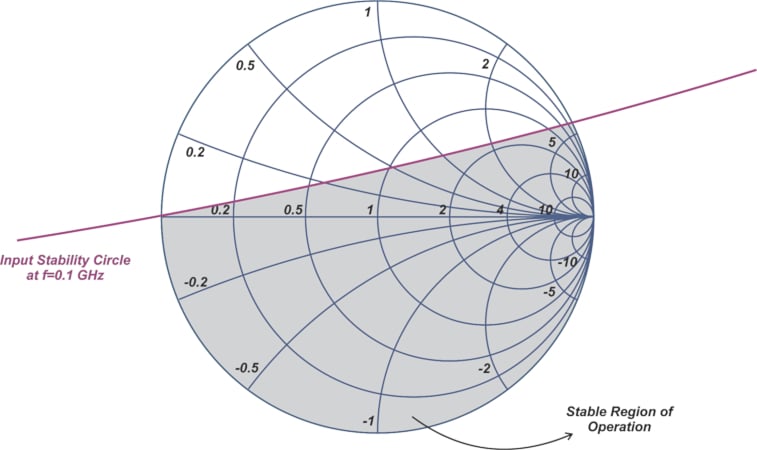
Figure 4. Stable region in the Γ_S plane.

 

Similarly, we can plot the output stability circle on a Smith chart to determine the usable Γ_L values, as demonstrated by Figure 5.

 

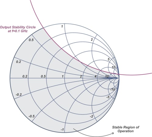
Figure 5. Stable region in the Γ_L plane.

 

Once again, the center of the Smith chart is used as a test point to determine the stable region of operation. At the center of the Smith chart, Γ_L = 0, and Equation 5 produces |Γ_IN| = |S₁₁|; from Table 1, we have |Γ_IN| = |S₁₁| = 0.72 at f = 100 MHz. Therefore, the center of the Smith chart belongs to the stable region of operation.

 

Possible Arrangements For a Potentially Unstable Device

There are several different ways a stability analysis can go wrong. To avoid them, we must exercise care in correctly interpreting the stability circles. In this section, we’ll take a look at some of the different possible arrangements.

When the stability circle intersects the Smith chart, the device is potentially unstable. In the above example, the magnitude of S₁₁ and S₂₂ was less than unity, so the center of the Smith chart produced a stable region of operation. When |S₁₁| > 1 or |S₂₂| > 1, the center of the Smith chart was in the unstable region of operation. Figure 6 shows the Γ_L plane for this case.

 

Figure 6. The stable region in the Γ_L plane when either (a) |S₁₁| < 1 or (b) |S₁₁| > 1.

 

It is also possible for the intersecting stability circle to enclose the center of the Smith chart. This produces the two arrangements seen in Figure 7.

 

Figure 7. The stable regions when the stability circle encloses the center of the Smith chart, for (a) |S₁₁| < 1 or (b) |S₁₁| > 1.

 

The stability circle might also be entirely inside the Smith chart (Figure 8). 

 

Figure 8. The stable regions when the stability circle both encloses the center of the Smith chart and is entirely inside the Smith chart. |S₁₁| < 1 in Figure 8(a). |S₁₁| > 1 in Figure 8(b).

As well as being inside the Smith chart, the stability circles in Figure 8 also enclose the Smith chart's center. However, it’s also possible for the stability circle to be inside the Smith chart and not enclose the chart's center.

Figures 6, 7, and 8 depicted output stability circles, which are plotted in the Γ_L plane. Similar situations are also possible in the Γ_S plane. Figure 9 illustrates a case where the input stability circle intersects the Smith chart but doesn’t enclose the center of the chart.

 

Figure 9. The stable region in the Γ_S plane when (a) |S₂₂| < 1 or (b) |S₂₂| > 1.

 

We’ve shown the input and output stability circles in separate diagrams, but it’s common to plot both stability circles on one Smith chart. If we do this, we must be extra careful to make sure we’re using the correct circle when analyzing the circuit’s stability behavior.

 

Possible Unconditionally Stable Device Arrangements

In the above examples, some values of the termination produce an unstable operation. To have unconditional stability, the stability circle should either fall completely outside of the Smith chart or completely enclose the Smith chart. Figure 10 illustrates these two scenarios for the Γ_L plane.

 

Figure 10. Two possible arrangements for an unconditionally stable device.

 

If either |S₁₁| > 1 or |S₂₂| > 1, the network cannot be unconditionally stable; in these cases, either the termination Γ_L = 0 or Γ_S = 0 leads to unstable operation.

 

Featured image used courtesy of Adobe Stock; all other images used courtesy of Steve Arar