Demystifying the Skin Effect: Insights into AC Current Distribution
This article will demonstrate that the AC current density decreases exponentially into a conductor. It will also explain why we can assume that the total current has a uniform distribution from the surface down to one skin depth of the conductor.
We previously learned that a time-varying current tends to mostly flow near the outer surface of the conductor—a phenomenon known as the skin effect. Superficially, the skin effect might be taught and remembered as AC current flowing mainly through the skin depth of the conductor. The reason I call this explanation superficial is that it might make us ignore the important underlying assumptions that are made to arrive at this approximation. The actual distribution of current, even in an isolated cylindrical conductor, can be much more nuanced than the above simple explanation.
For example, what is the current distribution if the radius of the cylindrical conductor is 2.5 times greater than the skin depth at the frequency of interest? To answer such questions, we need to take a closer look at the physics behind the skin effect and how the commonly used formula of skin depth is derived.
This article examines the skin effect in a conducting half-space. Building on these concepts, the next article in this series will take a look at the current distribution in conductors of circular cross-sections as well.
Skin Effect and EM Wave Propagation in Good Conductors
The skin effect is related to a basic electromagnetics problem: the propagation of electromagnetic waves in a good conductor. If you look into any reputable textbook on electromagnetic theory, you’ll see that the problem of wave propagation in a good conductor is usually the starting point of introducing the skin effect.
This problem is first analyzed for a homogeneous conductor of infinite depth and length. Skipping some of the mathematical steps, in the next section, we’ll investigate wave propagation in a conductive half-space.
Wave Propagation in a Homogeneous Conducting Half-Space
Figure 1 shows a homogeneous conductor of infinite depth and length that occupies half the space (it occupies -∞ < x < +∞, -∞ < z < +∞, and y ≥ 0). The question is, how does an electromagnetic wave penetrate this conductive block?
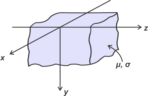
Figure 1. Representation of conducting material filling half of the 3D space
Like many other electromagnetics problems, textbooks examine the propagation of a plane wave in this conducting half-space. Plane waves are a simplified idealization of real-world electromagnetic waves, but they can still help us develop a useful understanding of the behavior of EM waves in general.
In a plane wave, electric (E) and magnetic fields (H) are perpendicular to one another and to the direction of propagation—we call them transverse electromagnetic waves (or TEM waves). Also, in a plane wave, every point on planes perpendicular to the direction of propagation “sees” the same electric and magnetic fields.
Let’s take the example of Figure 2. Let’s assume that just above the surface of our semi-infinite conductive block, the electric field (E) is in the z-direction, and the magnetic field (H) is in the x-direction. Therefore, the wave propagates in the y-direction.
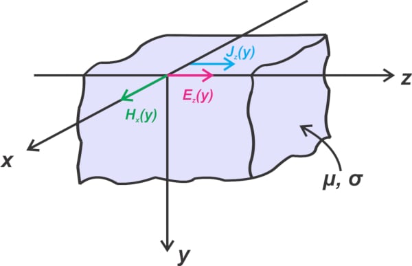
Figure 2. Electric field, magnetic field, and current density in a semi-infinite conductive block
Since E and H are respectively in the z- and x-directions, they are denoted as Ez and Hx in the figure. With the assumption of being a plane wave, the electric and magnetic fields are constant on the planes perpendicular to the direction of propagation, i.e., the planes perpendicular to the y-axis. This means that the electric and magnetic fields don’t change with x or z. That’s why the above figure shows Ez and Hx as a function of y only.
Also, in a good conductor, the current density, J, and the electric field, E, are in the same direction and are related by J = σE, where σ is the conductivity of the conductor. Therefore, in our problem, the vector J has only one component in the z-direction, denoted by Jz(y) in the figure.
All of these assumptions and considerations simplify the problem and allow us to easily solve Maxwell’s equations to arrive at the current density equation as follows:
\[J_z(y)=J_0 e^{-\frac{y}{\delta}}e^{-j\frac{y}{\delta}}\]
Equation 1
You can find the derivation of the above equation in Introductory Electromagnetics by Z. Popovic. In Equation 1, J0 is the magnitude of the current density at the surface of the conductor; and δ is the skin depth given by:
\[\delta = \frac{1}{\sqrt{\pi f \mu \sigma}}\]
Equation 2
Equation 1 means that the amplitude of the current density at the skin depth (at y = δ) decreases to 1/e of its value at the surface of the conductor. Figure 3 should give you an initial idea of how the current density changes with y at a given instant in time (we’ll shortly make a correction to this waveform!).
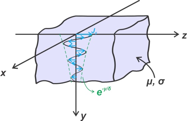
Figure 3. Current density decreases with increasing depth into the conductive block
Note that, due to the second exponential term in Equation 1, the current density also undergoes a significant phase shift with respect to the current density at the surface of the conductor. The exponential term e-jy/δ produces a phase lag of 1 radian (or about 57 degrees) at a depth of y = δ.
Also, this exponential term equals -1 at y = πδ, which shows that the current direction at particular depths can reverse with respect to the direction at the surface of the conductor.
How Large Is the Skin Depth in Comparison to the Wavelength?
It’s instructive to compare the skin depth with the wavelength inside the conductor. From Equation 1, we observe that the attenuation constant ⍺ and phase constant β of a good conductor are both equal to the reciprocal of the skin depth δ:
\[\alpha = \beta = \frac{1}{\delta}\]
Equation 3
Also, we know that the wavelength is given by:
\[\lambda= \frac{2 \pi}{\beta}\]
Equation 4
Combining equations 3 and 4 produces:
\[\lambda= 2 \pi \delta\]
Equation 5
This result is kind of interesting if you think about it. It says that one wavelength in the conductor is about 6 times larger than the skin depth. Therefore, the wave is significantly attenuated at a distance equal to one wavelength.
Substituting λ = 2πδ in the first exponential term in Equation 1, we observe that the wave amplitude can be reduced to a value of e-2π ≈ 0.002 in just one wavelength. Therefore, the waveform in Figure 3 is not 100% correct, as it shows that the signal gets attenuated only gradually over one wavelength.
To plot the current density waveform, we can find the instantaneous expression of the current density from its phaser value in Equation 1:
\[J(y,t)=Re [ J_z(y)e^{j \omega t}] = \Big ( J_0 e^{-\frac{y}{\delta}} cos \big ( \omega t- \frac{y}{\delta} \big ) \Big )\overrightarrow{a_z}\]
Equation 6
To more easily interpret the plot, we can use Equation 3 to express the above equation in terms of y/λ. The plot of the amplitude of J(y, t) versus y/λ at the t = 0 instant is provided in Figure 4 (blue curve).
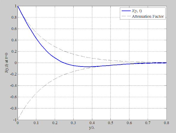
Figure 4. Amplitude of the current density versus depth represented as a fraction of a wavelength
The dashed lines in Figure 4 are the envelope of the waveform obtained from the attenuation term e-y/δ. As can be seen, the wave amplitude gets heavily attenuated at depths less than one wavelength.
To summarize, the above discussion shows that the current density reduces exponentially and is not uniform in the skin depth of the conductor. It also doesn’t abruptly fall to zero at depths larger than the skin depth. At the skin depth, it is reduced by a factor of e-1 = 0.37. So why do we assume that the AC current is uniformly distributed in the skin depth of the conductor? Read on to learn the reason for this!
Modeling the AC Resistance of Conductors
As electronics engineers, we’re mainly interested in developing a circuit model for different physical phenomena. This is also true in the case of the skin effect. Rather than dealing with electromagnetics, we prefer to use the skin effect concept to determine the equivalent resistance of conductors at high frequencies.
Having the AC resistance, we can find the conductor losses and determine how a signal traveling through the conductor is going to get attenuated. To find the equivalent AC resistance, we consider a volume of the conductor with length l and depth d, as shown in Figure 5 below.
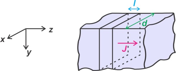
Figure 5. Volume of a conductor with length L and depth d
We need to find the voltage drop in the length, l, and divide it by the total current flowing through the cross-sectional area of the conductor. The potential difference across a length, l, at the surface of the conductor is ΔV = E0l, where E0 is the amplitude of the electric field at the surface. Applying J = σE, we have:
\[\Delta V = \frac{J_0l}{\sigma}\]
Equation 7
The total current flowing through the cross-sectional area of the conductor can be found by integrating Jz(y) over 0 ≤ y < ∞ and depth d. This step involves one of the most important assumptions of the simplified skin depth approximation. To make it easier to understand, I’ll take the integral over 0 ≤ y
\[\begin{eqnarray}
I &=& d \int_{0}^{t} J_z(y) = d \int_{0}^{t} J_0 e^{-\frac{y}{\delta}}e^{-j\frac{y}{\delta}} dy \\
&=& \frac{d J_0 \delta}{1+j} \Big ( 1 - e^{-t(1+j)/\delta} \Big )
\end{eqnarray}\]
Equation 8
Note that since the current is only a function of y, I’ve simply multiplied the result of the integral over y by the factor d. Taking the limit as t goes to infinity, we have:
\[I = \frac{d J_0 \delta}{1+j}\]
Equation 9
Dividing Equation 7 for the voltage by Equation 9 for the current gives us the impedance of the conductor:
\[Z = \frac{\Delta V}{I} = \frac{l}{\sigma d \delta} (1+j)\]
Equation 10
As can be seen, the conductor impedance has both resistive and inductive components. Here, the resistive part, which causes conductive losses in transmission lines, is of interest to us:
\[R = \frac{l}{\sigma d \delta}\]
Equation 11
This is the resistance of a length l of the conductor with depth d that extends from y = 0 to y = ∞. The above equation might remind you of the familiar equation of DC resistance below:
\[R_{DC} = \frac{l}{\sigma A}\]
Equation 12
where l and A are the length and cross-sectional area of the conductor.
Equating Equations 11 and 12, we have A = dδ. This means that rather than assuming that the current has a y-dependent distribution over y = 0 to y = ∞, we can assume that the total input current has a uniform distribution in one skin depth of the conductor. This is actually the same simplified explanation of the skin effect that we presented in the introduction of this article.
However, we now know the underlying assumptions. The key assumption here is that the conductor is a half-space. For Equation 9 (current, I) to be valid, the conductor should sufficiently extend in the positive y-direction so that the exponential term in the integral of Equation 8 can be neglected. The real-world conductors are not a half-space, but we use the above results to estimate their AC resistance. Such approximations can produce reasonably acceptable results only if the conductor’s radius of curvature is much larger than the skin depth so that it practically acts like a half-space for the electromagnetic waves.
In the next article, we’ll continue this discussion and take a look at the skin effect in cylindrical conductors. We’ll see how the ratio of the wire’s radius to the skin depth can significantly affect the current distribution in a round conductor.
Featured image used courtesy of Adobe Stock