Introduction to Dielectric Loss in Transmission Lines

Two of the most important loss mechanisms in transmission lines are conductor loss and dielectric loss. The conductor loss is influenced by the skin effect phenomenon that we introduced previously. The dielectric loss is related to the properties of the insulating material placed between the conductors. In this article, we’ll learn how the dielectric’s relative permittivity and loss tangent affect the performance of transmission lines.

 

Equivalent Circuit of a Transmission Line

The equivalent circuit of a two-conductor interconnect at high frequencies is shown in Figure 1.

 

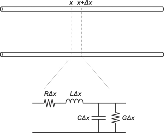
Figure 1. Equivalent circuit of a two-conductor transmission line.

 

As discussed in a previous article, the resistance R models the loss from the series resistance of the conductors, whereas the conductance G accounts for the dielectric loss. In other words, G characterizes the electromagnetic power that the dielectric absorbs and turns into heat. This effect becomes more pronounced at higher frequencies.

Before diving in too far, let’s review the characteristics of a lossless capacitor.

 

Ideal, Lossless Capacitor

Consider the familiar capacitance equation below:

$$C = \epsilon_0 \epsilon_r \frac{A}{d}$$

Equation 1

where:

• C is the capacitance
• ε₀ is the permittivity of free space
• ε_r is the relative permittivity of the dielectric material
• A is the parallel plate area
• d is the distance between the two conductive plates

 

The relative permittivity, ε_r, also known as the dielectric constant denoted by Dk, characterizes how well the dielectric material stores an electric field. The relative permittivity can be defined as the ratio of the capacitance that a capacitor produces with a given dielectric to that obtained when the same capacitor has vacuum as its dielectric.

The dielectric constant for most PCB materials is in the 2.5 to 4.5 range. Some ceramics, such as barium titanate, exhibit dielectric constants as high as 7,000. The dielectric constant generally decreases as frequency increases.

The admittance, Y, of an ideal capacitor is given by:

$$Y_{ideal}=jC \omega = j \epsilon_0 \epsilon_r \frac{A}{d} \omega$$

Equation 2

where:

• ω is the frequency in radians = 2πf

 

The relative permittivity, ε_r, is a real value; hence, a capacitor's admittance is a purely imaginary value. We can also see from this equation that the capacitor admittance is a function of frequency. Equation 2 shows that with a real ε_r, the current going through the capacitor leads the voltage waveform by precisely 90°, as illustrated in Figure 2.

 

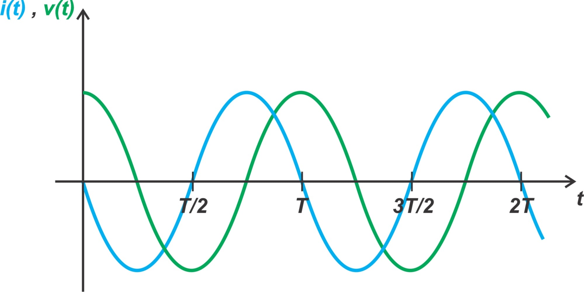
Figure 2. The phase relationship between voltage and current waveforms of an ideal capacitor.

 

It’s worth mentioning that the impedance and wave velocity of a transmission line are affected by the dielectric constant of the insulating material. Also, for an ideal capacitor, the average power dissipated is zero.

 

How Does a Dielectric Increase Capacitance?

Consider a dielectric made up of polar molecules. With polar molecules, there is a permanent separation between the center of positive and negative electric charges in the molecules. In the absence of an external electric field, the electric dipoles of the molecules are randomly oriented, as shown in Figure 3(a).

 

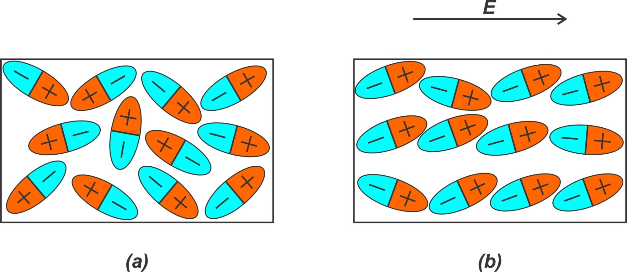
Figure 3. (a) Dielectric dipoles without an external electric field and (b) in the presence of an external field.

 

However, in the presence of an electric field, as in Figure 3(b), the dipoles experience a torque and partially align with the field. As you can see, the alignment of the electric dipoles leads to some induced surface charge of opposite polarity on the opposite faces of the dielectric. This behavior is the basic property that enables a dielectric to increase the capacitance of a capacitor.

To understand this, consider a charged capacitor with voltage V₀ and charge Q₀ on each plate, as Figure 4(a) depicts. The electric field between the plates is E₀. Assume that the capacitor is disconnected from its charging voltage source so that the charges are stuck on the plates and don’t have a path to discharge.

 

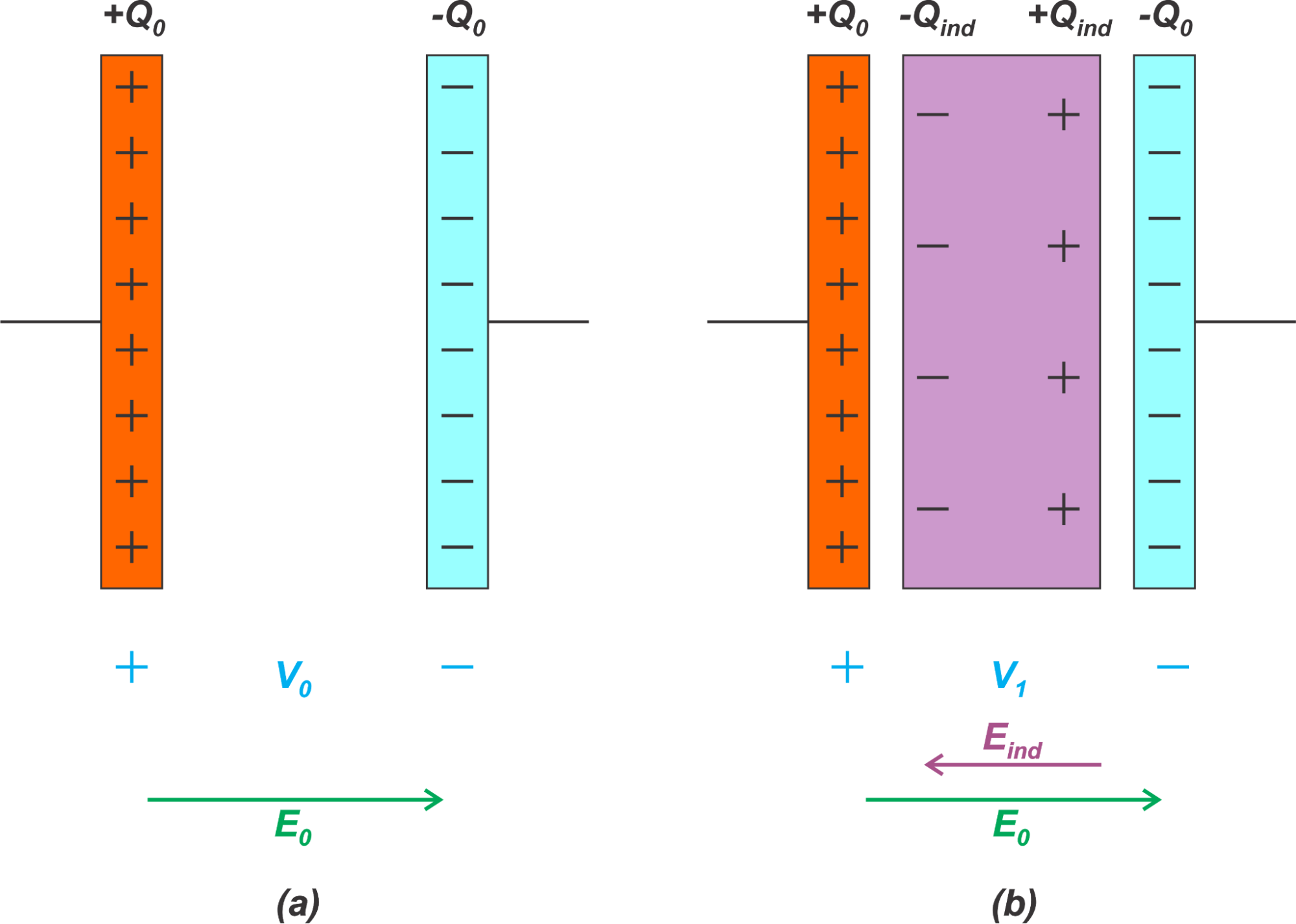
Figure 4. The impact of a dielectric on capacitor electric field

 

If we place a dielectric between the plates, as shown in Figure 4(b), the electric dipoles of the dielectric align with the external field and produce some induced surface charge on the opposite faces of the dielectric (Q_ind on the right face and -Q_ind on the left face). Note that the dielectric's negative surface charge faces the capacitor's positive plate and vice versa.

The induced surface charges produce an internal electric field that opposes the initial electric field between the capacitor plates. As a result, the overall electric field (which is equal to E₀ − E_ind) and the voltage between the capacitor plates are reduced (V₁ < V₀).

Note that the charge on the capacitor plates has not changed, but their contribution to the capacitor voltage is partially canceled by the surface charges of the dielectric. How are these changes going to affect the capacitance? This can be answered by considering the capacitance definition in Equation 3:

$$C= \frac{Q}{V}$$

Equation 3

 

We observe that the charge stored on the capacitor plates is the same while the voltage across the capacitor is reduced. This corresponds to an increase in the capacitance.

In the above discussion, we have assumed that the dielectric molecules are polar; however, a dielectric with nonpolar molecules also increases the capacitance. With a nonpolar dielectric, the external electric field produces some charge separation and an induced dipole moment. These induced dipoles then align in the direction of the external field, similar to the case of permanent dipoles.

 

Lossy Dielectrics

The interaction between the dielectric molecules and the external electric field can be much more complicated than the above discussion. For example, when a molecule is displaced from equilibrium by an electric field, the molecule can oscillate for a short time after removing the external field. Alternatively, the molecules may not be able to align at sufficiently high switching frequencies for the external electric field.

Two different types of motion can describe the overall motion of the dipoles. First, if the motion of the dipoles contributes to a current component that leads the capacitor voltage by precisely 90°, the dielectric increases the capacitance. Second, dipole displacements that lead to a current in phase with the capacitor voltage can be modeled by a resistive component. This latter type of dipole displacement actually contributes to the losses. This loss term is modeled as a parallel resistor (the conductance G in the transmission line model of Figure 1).

 

The Complex Dielectric Constant

As noted above, the dielectric constant of a lossless dielectric material is a real value. However, to completely describe the electrical properties of a lossy dielectric, we define ϵ_r as a complex value:

$$\epsilon_r = \epsilon_r ^{\prime} -j\epsilon_r ^{\prime \prime}$$

Equation 4

 

Combining Equation 4 with Equation 1, the admittance of a capacitor with a lossy dielectric is:

$$Y_{lossy}= j \epsilon_0 \epsilon_r^{\prime} \frac{A}{d} \omega + \epsilon_0 \epsilon_r^{\prime \prime} \frac{A}{d} \omega$$

Equation 5

 

By assuming a complex dielectric constant, two terms appear in this admittance equation. The imaginary part of the admittance corresponds to an ideal lossless capacitor, whereas the real part of the admittance accounts for the dielectric loss.

Losses of the dielectric material are usually expressed by the dielectric loss tangent or sometimes simply the loss tangent, which is defined as the ratio of the real and imaginary parts of the permittivity:

$$\tan(\delta) = \frac{\epsilon_r ^{\prime \prime}}{\epsilon_r ^{\prime}}$$

Equation 6

 

The loss tangent at various frequencies can be found in various handbooks. PCB laminate data sheets also provide a dielectric loss tangent value and a Dk value. By multiplying these two values together, we can find the imaginary part of the dielectric constant using Equation 6.

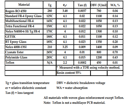
The characteristics of some common PCB laminates are listed below in Table 1. For a dielectric to be classified as low loss, the loss tangent should be below 0.004.

 

Table 1. Characteristics of common PCB laminates. Data used courtesy of Altium

 

Frequency Dependence of Dielectric Properties

The dielectric constant's real and imaginary parts can vary to some extent with frequency. This is illustrated in Figure 5 below. The figure also highlights that there are several different dielectric loss mechanisms that dominate at different frequencies.

 

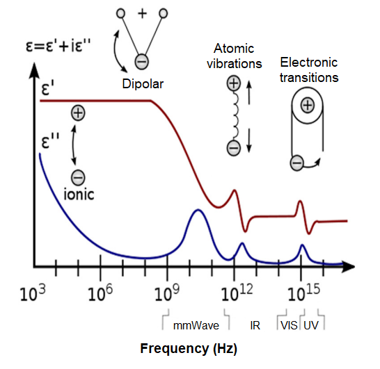
Figure 5. Dielectric constant real and imaginary components as a function of frequency. Image used courtesy of Dr. Ken Mauritz

 

Finding the Conductance of a Transmission Line

Now, we can use Equation 5 to find an expression for the conductance G in our transmission line model:

$$G = \epsilon_0 \epsilon_r^{\prime \prime} \frac{A}{d} \omega$$

Equation 7

 

The above expression can be simplified by noting that the line’s capacitance is given by:

$$C = \epsilon_0 \epsilon_r^{\prime} \frac{A}{d}$$

Equation 8

 

Combining these two equations with Equation 4 produces:

$$G = C tan(\delta ) \omega$$

Equation 9

 

From Equation 9, we can see that the conductance is directly proportional to the capacitance, loss tangent, and frequency.

 

The Impact of Dielectric Loss on Signal Transmission

Hopefully, this has provided you with a better understanding of dielectrics, including the importance of relative permittivity and loss tangent. In the next article in this series, we’ll expand on this discussion and see how the above results can be used to characterize the effect of dielectric loss on the signal attenuation as it travels down the line.

 

Unless otherwise noted, all images are the author's.