Interference, Pre-Emphasis, and the Capture Effect in FM and PM Systems

This article explores how interference impacts frequency and phase modulation (FM and PM) systems. It then highlights how the pre-emphasis/de-emphasis (PDE) technique enhances FM’s resilience to interference. The article concludes with a discussion of the FM capture effect and a comparison between FM and amplitude modulation (AM) in terms of interference suppression.

 

Interference in FM Systems

We understand that the noise power at the FM receiver output is concentrated at higher frequencies. Much like noise, interference becomes increasingly significant at higher frequencies in FM transmission. In other words, high-frequency components are more susceptible to interference. To understand this, we’ll examine how the simplified FM demodulation system illustrated below reacts to an interfering component.

 

Figure 1. Simplified FM demodulation system.

 

Consider an unmodulated carrier described by the equation:

$$s(t) = A_c\cos(\omega_c t)$$

Equation 1.

where:

A_c is the amplitude of the carrier

ω_c is its angular frequency

Assume that the interference component i(t) is a sinusoid of amplitude I and frequency ω_c + Δω, i.e. i(t) = I cos[(ω_c + Δω)t]. Therefore, the overall corrupted signal is:

$$r(t) = A_c\cos(\omega_c t) + I\cos\left[(\omega_c + \Delta\omega)t\right]$$

Equation 2.

 

The discriminator extracts the time derivative of the phase of the above signal. To obtain the phase, we utilize fundamental trigonometric identities to rewrite r(t) as:

$$r(t) = \left[A_c + I\cos(\Delta\omega t)\right]\cos(\omega_c t) - I\sin(\Delta\omega t)\sin(\omega_c t)$$

Equation 3.

 

Equation 3 can be simplified into a single sinusoidal function using amplitude-phase form. Specifically, the expression A cos(x) + B sin(x) is equal to R cos(x − θ) where R and θ are given by:

$$R = \sqrt{A^2 + B^2} \quad \text{and} \quad \theta = \tan^{-1}\left(\frac{B}{A}\right)$$

Equation 4.

 

As we conduct the FM signal analysis, our interest lies only in the phase of the input signal r(t), which can be obtained using the above identity as:

$$\theta = \tan^{-1}\left(\frac{I\sin(\Delta\omega t)}{A_c + I\cos(\Delta\omega t)}\right)$$

Equation 5.

 

When the interfering signal amplitude I is much smaller than the carrier amplitude A_c, the phase expression simplifies to:

$$\theta \approx \tan^{-1}\left(\frac{I\sin(\Delta\omega t)}{A_c}\right) \approx \frac{I}{A_c}\sin(\Delta\omega t)$$

Equation 6.

 

Finally, by taking the time derivative of θ, we obtain the discriminator output voltage as:

$$v_{out} = k_d\frac{d\theta}{dt} = k_d \times \frac{I\Delta\omega}{A_c}\cos(\Delta\omega t)$$

Equation 7.

 

where k_d is the gain factor of the discriminator. Figure 2 plots the amplitude of the output voltage in terms of the frequency separation Δω.

 

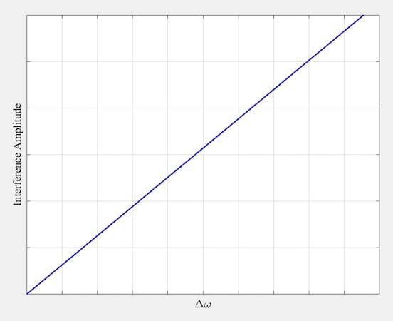
Figure 2. Plot of the interference output against Δω.

 

Now, let's consider the implications of the analysis above.

 

Insight into the Analysis Results

First, the input was an unmodulated carrier, so whatever we observe at the discriminator output is caused by the interference signal. Second, as shown in Equation 7, the interference-induced output is a sinusoid at the frequency Δω—the frequency separation between the carrier at ω_c and the interfering signal at ω_c + Δω. Furthermore, the amplitude of the output sinusoid grows linearly with Δω.

Initially, it may seem counterintuitive that an interferer farther from the carrier frequency produces a stronger response at the discriminator output. To clarify this, consider the phasor representation of the summation in Equation 2, illustrated below.

 

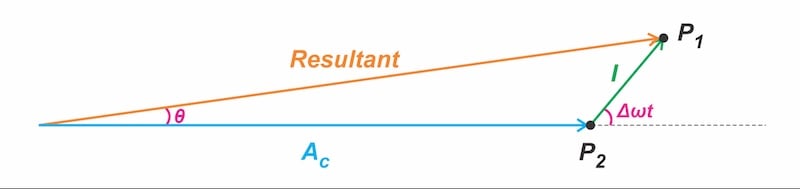
Figure 3. Phasor diagram showing the carrier (blue) and interference (green); the orange curve depicts the overall, corrupted input.

 

The carrier (blue) serves as the phase reference, giving the interference vector (green) a phase of Δωt. As time progresses, the interference vector rotates around the carrier vector’s tip P₂, continuously altering the resultant vector’s phase θ. At a higher offset frequency Δω, the interference vector rotates more rapidly, leading to faster phase variations in the overall corrupted signal (as captured analytically in Equation 6). Since the discriminator acts as a differentiator, it yields larger outputs for more rapid input variations, explaining the heightened impact of interference at higher frequency offsets.

 

The PDE Impact on Interference Behavior

How does the interference response change when we use a de-emphasis filter? As the interference signal passes through the de-emphasis filter, its amplitude is altered according to the filter’s magnitude response. Due to its lowpass nature, the de-emphasis filter attenuates high-frequency components that lie outside its passband. This leads to the typical interference characteristic shown below.

 

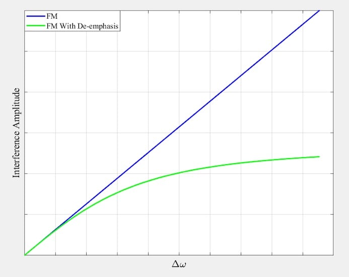
Figure 4. Interference output versus Δω for FM systems without (blue) and with (green) de-emphasis.

 

A first-order de-emphasis filter attenuates high frequencies proportionally to 1/f, flattening FM’s interference response at the upper end. Therefore, the PDE technique enhances the system’s resilience against both noise and interference.

 

Interference in PM Systems

At this stage, it’s also useful to examine how interference affects phase-modulated (PM) signals. The previous analysis remains applicable, with the key distinction that an ideal phase demodulator extracts the instantaneous phase of the input signal, rather than its time derivative. Hence, the phase demodulator output is proportional to the phase term θ defined in Equation 6, leading to:

$$v_{out} = k_d \times \theta \approx k_d \times \frac{I}{A_c}\sin(\Delta\omega t)$$

Equation 8.

 

With the PM scheme, the output amplitude is independent of the frequency separation Δω (see Equations 7 and 8 for comparison). Figure 5 compares the interference response of PM with that of FM, both with and without de-emphasis.

 

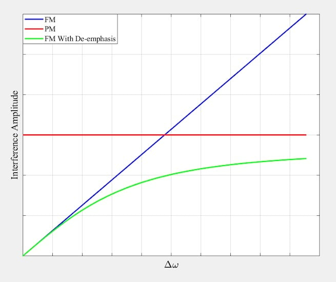
Figure 5. Interference output versus Δω for PM (red), FM without de-emphasis (blue) and FM with de-emphasis (green).

 

FM provides stronger interference rejection at low offset frequencies, while PM performs better at higher offsets. FM with de-emphasis effectively merges FM and PM characteristics. At low frequency offsets, it behaves like FM, while at higher offsets it resembles PM, yielding an interference response that remains nearly constant at high offset frequencies.

Note that although the figure suggests FM with de-emphasis yields a lower output than PM in the flattened region, this behavior might not be the case in general. The high-frequency value of the de-emphasized FM curve depends on the de-emphasis filter’s corner frequency and may sit higher or lower than PM depending on the chosen parameters.

Note that interference at offset frequencies beyond the message bandwidth is generally negligible, since such components are filtered out by a lowpass stage that follows the discriminator (see the block diagram in Figure 1).

 

FM Behavior in the Presence of Strong Interference

In the preceding analysis, we assumed that the interference amplitude I is much smaller than the carrier amplitude A_c. When this condition is violated, the system exhibits undesired behavior essentially akin to the below-threshold operation previously discussed in the FM noise analysis. To gain qualitative insight into this phenomenon, we turn once again to the phasor diagram. Figure 6 depicts the case where the interference amplitude is comparable with that of the carrier, and Δωt is close to π radians.

 

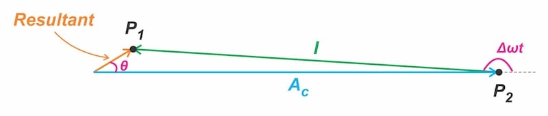
Figure 6. Phasor representation of a scenario where the interference and carrier amplitudes are comparable and Δωt is close to π radians.

 

Figure 7 illustrates how the phase θ of the resultant vector evolves over time, using example parameters A_c = 1, I = 0.9, and Δω = π radians/s.

 

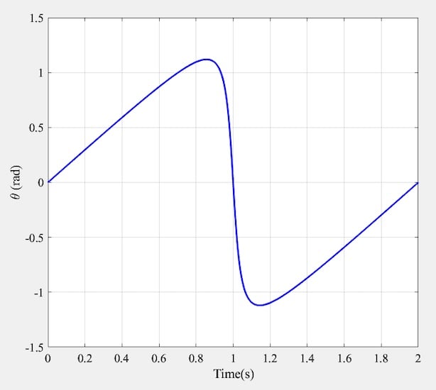
Figure 7. Plot of the resultant vector’s phase θ.

 

Note how a small phase shift in the interference around t = 1 s (or equivalently Δωt = π radians) triggers a sharp negative change in the resultant vector’s phase θ. This abrupt shift produces a negative spike at the discriminator output, which reflects the time derivative of the input phase. Figure 8 plots this derivative, showing how the derivative of θ evolves over time.

 

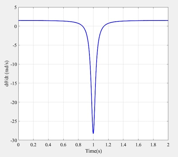
Figure 8. Plot of the time derivative of θ.

 

Such spikes are undesirable because they manifest as audible clicks on an FM receiver. When frequent, the individual clicks blend into a sustained crackling noise that obscures the intended signal. Therefore, FM systems are typically designed to avoid operation near the threshold region.

 

Capture Effect

Equations 7 and 8 reveal that interference output in angle-modulated systems decreases as the carrier amplitude A_c increases. Unlike angle modulation, AM systems exhibit interference levels that are independent of the carrier amplitude. As a result, angle-modulated systems have a distinct advantage over AM in suppressing weak interference.

Because FM systems tend to suppress weak interfering signals, a phenomenon known as the capture effect occurs when two transmitters operate with carrier frequencies separated by less than the audio bandwidth. If one signal exceeds twice the amplitude of the other, the stronger signal captures the channel and completely suppresses the weaker one. When two FM stations transmit signals of roughly equal amplitude, the receiver may initially capture one signal and then switch to the other. For instance, while driving along a highway, the car FM radio may abruptly lose one FM broadcast to another, then regain it just as quickly, depending on the car’s position and which signal dominates locally.

Unlike FM, which suppresses weaker signals, AM receivers pick up both signals when two stations use closely spaced carrier frequencies. The stronger signal may be more intelligible, but the weaker one remains audible. When both are similar in amplitude, mutual interference can render both unintelligible.

 

Wrapping Up

In this article, we examined how interference affects FM and PM systems, and how the PDE technique enhances FM’s ability to suppress it. We saw that PDE introduces hybrid behavior in FM, improving its performance across different frequency offsets. Finally, we explored the FM capture effect and highlighted FM’s advantage over AM in rejecting weak interference.