Technical Article

How to Perform Transient Analysis and Noise Source Simulation with LTspice

May 23, 2019 by Stephen Colley

Learn multiple ways to simulate noise sources—for both transient and noise analysis—in LTspice.

In a previous article, we discussed some examples of modeling noise in LTspice. Now, let's discuss how to build noise sources in the frequency domain using noise analysis and in the time domain using transient analysis. We'll do this by simulating circuit noise in LTspice.

This article assumes experience with the transient and noise analysis options found in the “Simulation->Edit Simulation Command” menu and some knowledge of noise in circuit components such as resistors.

Simulation 1: Sources for Noise Analysis in the Frequency Domain

In a noise analysis, LTspice uses all the noise sources it finds in circuit components such as resistors, transistors, and op-amps. This is sufficient for many analysis tasks, but sometimes a separate, independent noise source is useful. For example, a noise source may be part of a sensor. No standard signal source is available for noise analysis. To that bold statement, I add “that I know of and is documented!” If you know of one built into LTspice, please let us know in the comments section at the end of the article.

We start with a new, special number: 60.328×10¹⁸. Don’t worry, it will not be on the test. This is the value of a resistor that LTspice thinks will produce 1.000001 V/Hz^1/2 of thermal noise. You can get the same number if you use a lot of significant figures in the thermal noise calculation of a resistor, i.e., $$\sqrt{4k_{B}TR}$$. The key to the source described here is using a resistor as a white noise generator.

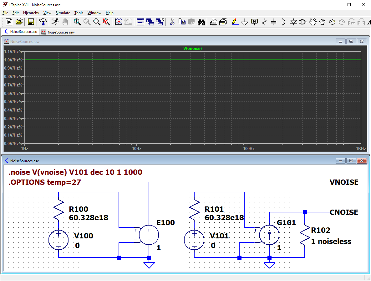
The voltage noise produced by the resistor is the input to a voltage-dependent voltage source. This part is “e” in the LTspice component library. The “e” source here uses a value of 1 to produce a source with an output of 1 V/Hz^1/2. Changing the value to 0.001 produces 1 mV/Hz^1/2 and so on. Another resistor with the same value is applied to the input of a voltage-dependent current source (“g” in the library) to produce current noise.

The "Noiseless" Feature in LTspice

Here is some detail about this circuit. R102 is there to convert the current noise to a voltage for plotting. It should be removed when a real load is used.

R102 is assigned the undocumented component attribute “noiseless”, which tells LTspice to ignore the resistor as a noise source. This feature is very useful because the extra noise from resistors does not have to be subtracted from the measurement.

The noiseless attribute is added using the Component Attribute Editor brought up by holding down the control key and right-clicking on the resistor body. Add the word “noiseless” as an additional value. Double click on the visible field to have it show as an additional value on the schematic.

I call the current output “cnoise” instead of “inoise” to avoid confusion with “inoise” used by LTspice as a special label. V100 and V101 are input sources that are required for a noise simulation.

Simulation 2: Using Random Functions in the Time Domain

Now we move over to the time domain and transient analysis. In the time domain, we need to produce the “fuzzy” waveforms we call noise. The sources shown here produce an approximation of “white” noise. We will take a “deep dive” into the pseudo-random functions in LTspice and explore them in detail.

Built into LTspice are Arbitrary Behavioral Voltage or Current Sources. They are called “B” functions, and we will use “bv” from the library. The current source is “bi”. B sources use a function to specify the output. There are three functions in LTspice that produce “noisy” or random numbers used as input to these sources.

The three functions are RAND( ), RANDOM( ), and WHITE( ). They produce pseudo-random numbers with different characteristics.

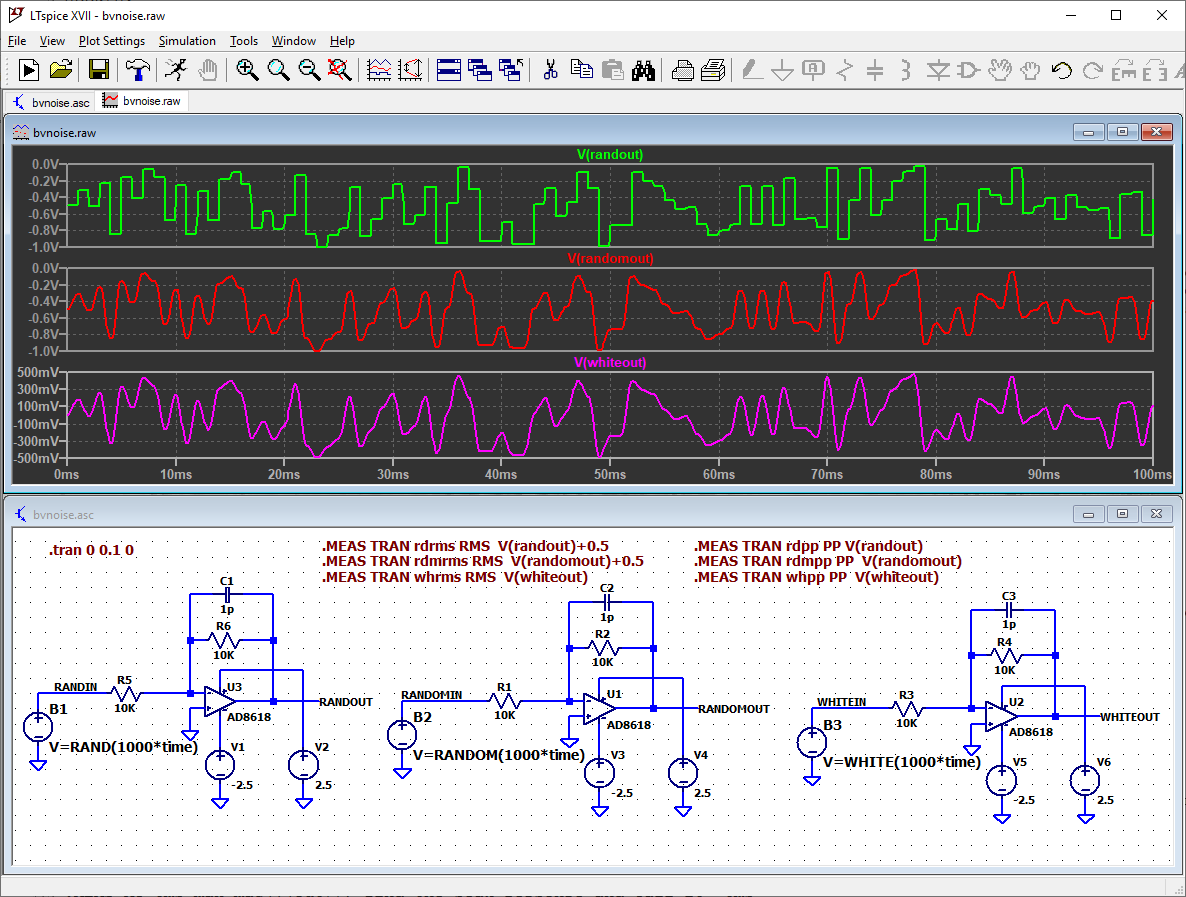
The figure shows an inverting amplifier repeated three times. Each instance uses one of the three functions. The time-domain plots show the differences in the outputs. RAND( ) is the top plot. The output is not smoothed and does not look like the “fuzzy” waveform we want. The middle plot is RANDOM( ). RANDOM( ) smooths the output but notice the DC offset. The bottom plot is WHITE( ). The output is a bit smoother and there is no DC offset.

Caution! The three sources produce correlated outputs. In other words, they move together. In an accurate noise simulation, all sources would be independent or uncorrelated. The internal random number generators are producing similar outputs, presumably because all the functions are based on the same time variable. If you need multiple, uncorrelated noise sources, a PWL source (described below) may be better.

The simulation includes .MEASURE directives that print the RMS and peak-to-peak values of the waveforms to the SPICE Error Log. Here are the results for this run.

whrms: RMS(v(whiteout))=0.238969 FROM 0 TO 0.1
rdmrms: RMS(v(randomout)+0.5)=0.247377 FROM 0 TO 0.1
rdrms: RMS(v(randout)+0.5)=0.27391 FROM 0 TO 0.1
whpp: PP(v(whiteout))=0.97515 FROM 0 TO 0.1
rdmpp: PP(v(randomout))=0.975855 FROM 0 TO 0.1
rdpp: PP(v(randout))=0.975857 FROM 0 TO 0.1

“wh--” is WHITE( ). “Rdm--” is RANDOM( ). “Rd--” is RAND( ). The peak-to-peak should be close to 1 volt. The ratio of peak-to-peak to RMS should be from 4 to 6, which is typical for white noise. Note that the offset is removed from RAND( ) and RANDOM( ).

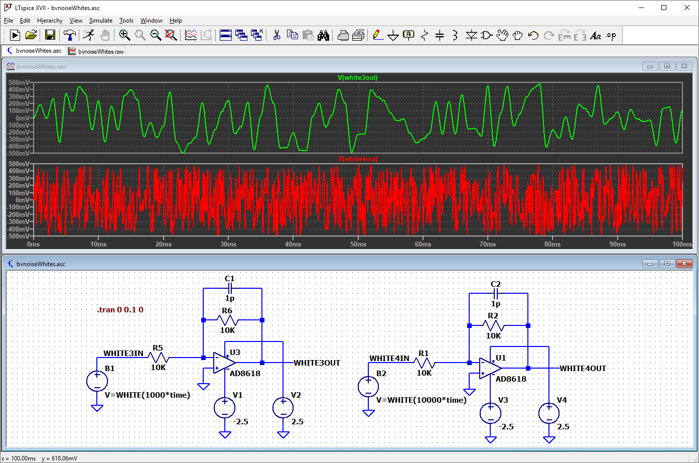
The high-frequency cutoff of the source is controlled by passing the function the internal “time” variable multiplied by a scale factor. A lot of this stuff is not documented. Experiment! Here are two plots showing scale factors of 1,000 and 10,000.

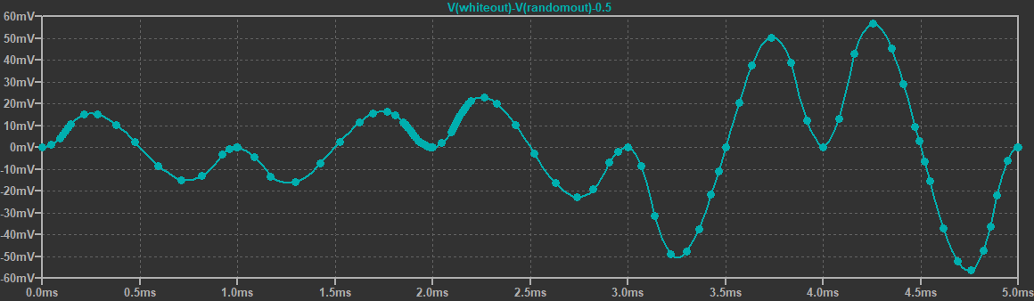
Let’s have a look at the outputs in more detail. Here are the first few milliseconds of the plots, with the data points highlighted.

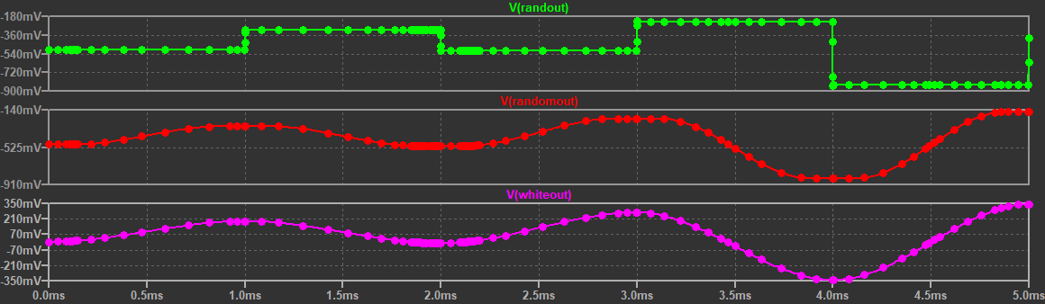
Sometimes RANDOM( ) and WHITE( ) are described as “low-pass-filtered” versions of RAND( ). These detailed plots show that this is not the case. Also, WHITE( ) is not just an offset version of RANDOM( ). Here is the difference of the two functions with the offset subtracted. The difference is substantial.

Simulation 3: Using PWL in the Time Domain

Another time-domain technique uses a PWL (Piecewise Linear) source. The segments of the waveform are specified with a list of time-voltage pairs in a text file. Here is the beginning of a 1,000 point file that I created with a spreadsheet and the RND( ) function. The output of RND( ) is offset by -0.5 to center the numbers around 0. Most spreadsheet programs should accept “=RND( )-0.5”.

0.001     0.2054203753
0.002     0.4484326853
0.003     0.1923825948
0.004     0.01742015759
0.005    -0.1907726361
0.006    -0.1055641709
0.007     0.4320814403
0.008     0.08668131624
0.009    -0.02411717432
0.010     0.006584482657
0.011    -0.1113930451

LTspice uses a white space separator. I used a tab. Put the file in the same directory as your schematic and enter the file name in the “PWL File” box when setting up the PWL function for the source. For example, I used “random_data.txt”.

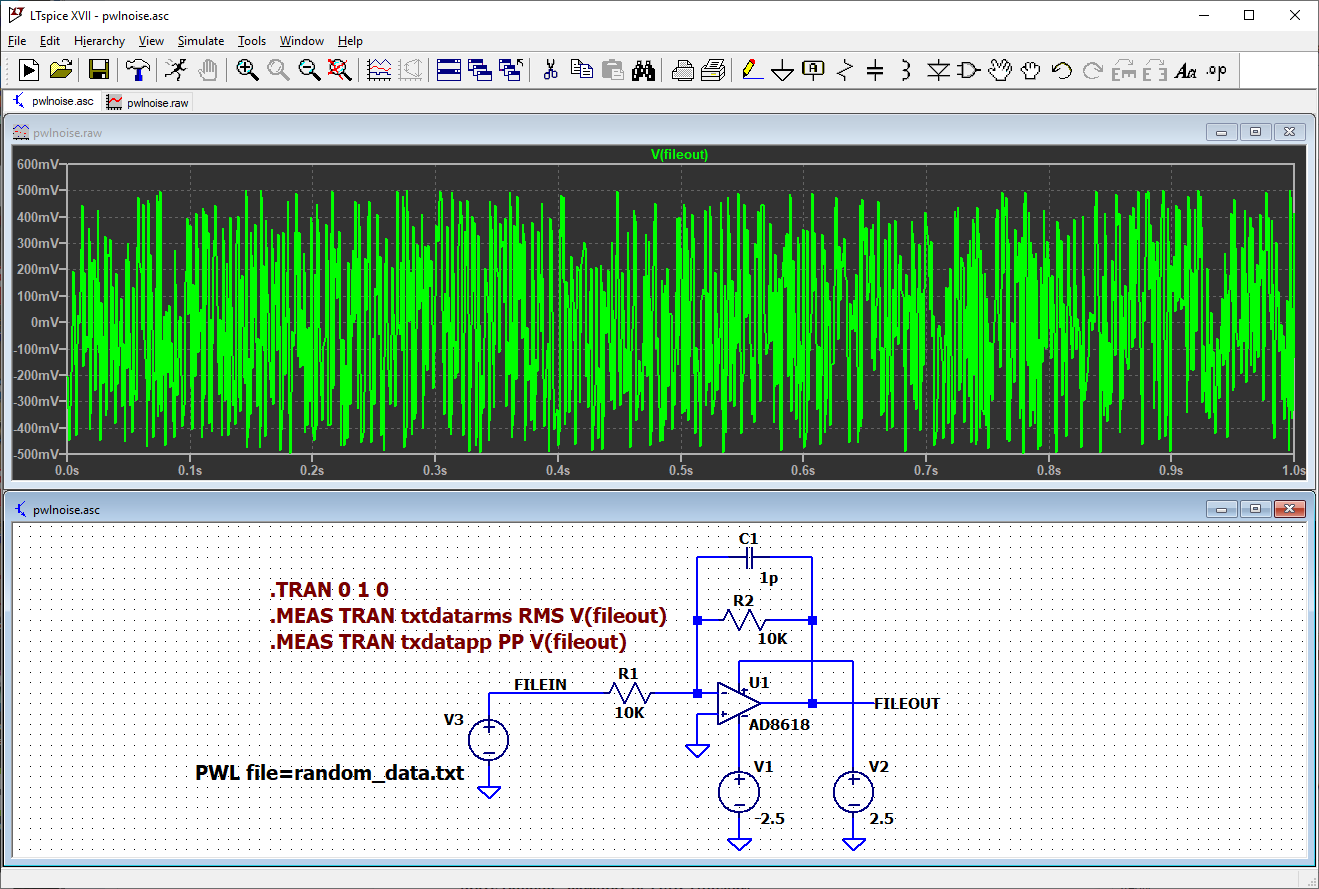
Here are the peak-to-peak and RMS measurements for this run.

txtdatarms: RMS(v(fileout))=0.233475 FROM 0 TO 1
txdatapp: PP(v(fileout))=0.998355 FROM 0 TO 1

Data from a run can be exported to a text file in the same format as the input file. See “File->Export data as text”. Here is the beginning of the exported file for this run. LTspice added an entry for time=0, which is not in the input file. The op-amp inversion and other circuit effects are seen when comparing the input and output files.

      time                      V(fileout)

0.000000000000000e+000        -2.023313e-001
1.000000000000000e-003        -2.023313e-001
2.000000000000000e-003        -4.453379e-001

Bonus Tip: Export into a .wav Audio File

LTspice can export plot data to a .wav audio file. Put this directive into the schematic above and produce one second of sound only an engineer could love.

.wave random_data.wav 16 44.1K V(fileout)

You have also produced a .csv to .wav file converter. Free!

Conclusion

The article presents several ways to simulate “white” noise sources and discusses some of their limitations. There are other creative ways to make noise sources for LTspice. For example, some people use semiconductor devices to create 1/ƒ noise. If you would like to share one, please comment below.