How to Create a Multilayer Perceptron Neural Network in Python

This is the 12th entry in AAC's neural network development series. See what else the series offers below:

1. How to Perform Classification Using a Neural Network: What Is the Perceptron?
2. How to Use a Simple Perceptron Neural Network Example to Classify Data
3. How to Train a Basic Perceptron Neural Network
4. Understanding Simple Neural Network Training
5. An Introduction to Training Theory for Neural Networks
6. Understanding Learning Rate in Neural Networks
7. Advanced Machine Learning with the Multilayer Perceptron
8. The Sigmoid Activation Function: Activation in Multilayer Perceptron Neural Networks
9. How to Train a Multilayer Perceptron Neural Network
10. Understanding Training Formulas and Backpropagation for Multilayer Perceptrons
11. Neural Network Architecture for a Python Implementation
12. How to Create a Multilayer Perceptron Neural Network in Python
13. Signal Processing Using Neural Networks: Validation in Neural Network Design
14. Training Datasets for Neural Networks: How to Train and Validate a Python Neural Network

In this article, we'll be taking the work we've done on Perceptron neural networks and learn how to implement one in a familiar language: Python.

Developing Comprehensible Python Code for Neural Networks

Recently I’ve looked at quite a few online resources for neural networks, and though there is undoubtedly much good information out there, I wasn’t satisfied with the software implementations that I found. They were always too complex, or too dense, or not sufficiently intuitive. When I was writing my Python neural network, I really wanted to make something that could help people learn about how the system functions and how neural-network theory is translated into program instructions.

However, there is sometimes an inverse relationship between the clarity of code and the efficiency of code. The program that we will discuss in this article is most definitely not optimized for fast performance. Optimization is a serious issue within the domain of neural networks; real-life applications may require immense amounts of training, and consequently thorough optimization can lead to significant reductions in processing time. However, for simple experiments like the ones that we will be doing, training doesn’t take very long, and there’s no reason to stress about coding practices that favor simplicity and comprehension over speed.

The entire Python program is included as an image at the end of this article, and the file (“MLP_v1.py”) is provided as a download. The code performs both training and validation; this article focuses on training, and we’ll discuss validation later. In any case, though, there’s not much functionality in the validation portion that isn’t covered in the training portion.

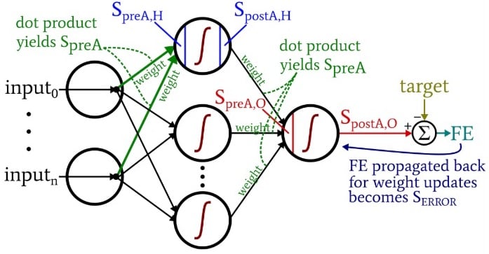
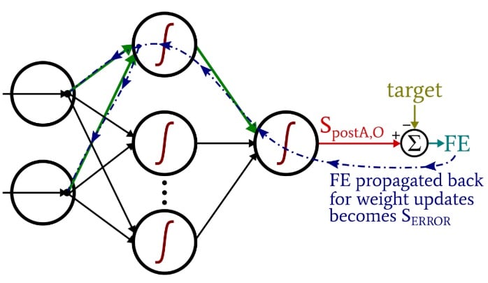
As you’re pondering the code, you may want to look back at the slightly overwhelming but highly informative architecture-plus-terminology diagram that I provided in Part 10.

Preparing Functions and Variables

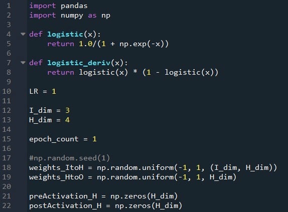
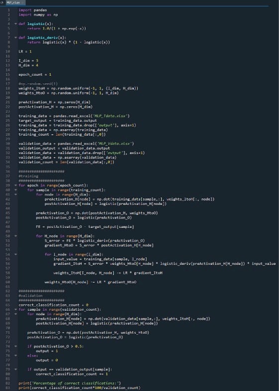
The NumPy library is used extensively for the network’s calculations, and the Pandas library gives me a convenient way to import training data from an Excel file.

As you already know, we’re using the logistic sigmoid function for activation. We need the logistic function itself for calculating postactivation values, and the derivative of the logistic function is required for backpropagation.

Next we choose the learning rate, the dimensionality of the input layer, the dimensionality of the hidden layer, and the epoch count. Training over multiple epochs is important for real neural networks, because it allows you to extract more learning from your training data. When you’re generating training data in Excel, you don’t need to run multiple epochs because you can easily  create more training samples.

The np.random.uniform() function fills ours two weight matrices with random values between –1 and +1. (Note that the hidden-to-output matrix is actually just an array, because we have only one output node.) The np.random.seed(1) statement causes the random values to be the same every time you run the program. The initial weight values can have a significant effect on the final performance of the trained network, so if you’re trying to assess how other variables improve or degrade performance, you can uncomment this instruction and thereby eliminate the influence of random weight initialization.

Finally, I create empty arrays for the preactivation and postactivation values in the hidden layer.

Importing Training Data

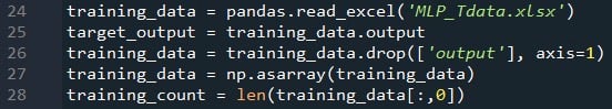
This is the same procedure that I used back in Part 4. I import training data from Excel, separate out the target values in the “output” column, remove the “output” column, convert the training data to a NumPy matrix, and store the number of training samples in the training_count variable.

Feedforward Processing

The computations that produce an output value, and in which data are moving from left to right in a typical neural-network diagram, constitute the “feedforward” portion of the system’s operation. Here is the feedforward code:

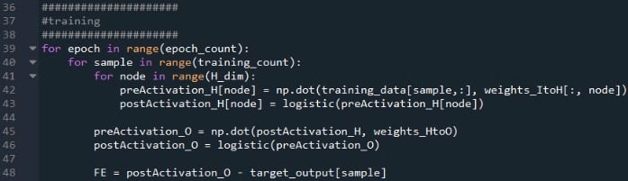
The first for loop allows us to have multiple epochs. Within each epoch, we calculate an output value (i.e., the output node’s postactivation signal) for each sample, and that sample-by-sample operation is captured by the second for loop. In the third for loop, we attend individually to each hidden node, using the dot product to generate the preactivation signal and the activation function to generate the postactivation signal.

After that, we’re ready to calculate the preactivation signal for the output node (again using the dot product), and we apply the activation function to generate the postactivation signal. Then we subtract the target from the output node’s postactivation signal to calculate the final error.

Backpropagation

After we have performed the feedforward calculations, it’s time to reverse directions. In the backpropagation portion of the program, we move from the output node toward the hidden-to-output weights and then the input-to-hidden weights, bringing with us the error information that we use to effectively train the network.

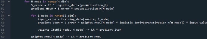
We have two layers of for loops here: one for the hidden-to-output weights, and one for the input-to-hidden weights. We first generate S_ERROR, which we need for calculating both gradient_HtoO and gradient_ItoH, and then we update the weights by subtracting the gradient multiplied by the learning rate.

Notice how the input-to-hidden weights are updated within the hidden-to-output loop. We start with the error signal that leads back to one of the hidden nodes, then we extend that error signal to all the input nodes that are connected to this one hidden node:

After all of the weights (both ItoH and HtoO) associated with that one hidden node have been updated, we loop back and start again with the next hidden node.

Also note that the ItoH weights are modified before the HtoO weights. We use the current HtoO weight when we calculate gradient_ItoH, so we don’t want to change the HtoO weights before this calculation has been performed.

Conclusion

It’s interesting to think about how much theory has gone into this relatively short Python program. I hope that this code helps you to really understand how we can implement a multilayer Perceptron neural network in software.

You can find my full code below:

Download Code