
How Is the Laplace Transform Used in Circuit Design?
In this article, we briefly review how the Laplace transform can help us solve circuits involving damped and steady-state sinusoidal signals.
In this Frequent Engineering Question (FEQ), we provide an at-a-glance overview of AC circuit analysis and design using the Laplace transform.
A common task in electrical engineering is to design and analyze circuits in which the currents and voltages continuously vary in a sinusoidal fashion.
When we are working with these types of circuits, we typically focus on the magnitude and phase of the signals rather than the continuous variations. We assume that the signals are and will always be sinusoids because components such as resistors, capacitors, and idealized amplifiers do not cause a signal to lose its sinusoidal shape.
These components do, however, influence a signal’s magnitude and phase.
Analyzing Circuits with Phasors
A common method of analyzing circuits with respect to magnitude and phase is the use of phasors, which are complex numbers that represent sinusoidal electrical signals.
When we are performing phasor analysis, we are working in the frequency domain, and expressions for current or voltage are written as functions of jω, where j is the imaginary number and ω is the angular frequency. Phasors help us to solve circuits involving steady-state sinusoidal signals.
Damped and Steady-State Sinusoids
The Laplace transform extends this approach by incorporating damped as well as steady-state sinusoids. It converts a function of time, f(t), into a function of complex frequency. We use the letter s to denote complex frequency, and thus f(t) becomes F(s) after we apply the Laplace transform. Complex frequency is defined as follows:
$$s = \sigma + j\omega$$
where σ is a constant that influences the way in which the magnitude of the sinusoid changes. No damping occurs when σ = 0.
Electrical engineers typically work with steady-state sinusoids rather than damped sinusoids. This allows us to assume that s = jω, and we can produce the Laplace transform of a signal simply by taking the F(jω) expression and replacing jω with s.
The Laplace Transform in AC Circuit Analysis
The Laplace transform is widely used in the design and analysis of AC circuits and systems. We can express currents, voltages, and impedances as functions of s. For example, the impedance of a capacitor can be written as
$$Z_C(s)=\frac{1}{sC}$$
We often write input-output relationships as functions of s. The transfer function of a low-pass filter, for example, can be expressed as follows:
$$T(s)=\frac{a_O}{s+\omega _O}$$
We also perform graphical analysis of a transfer function by plotting its poles and zeros on something called the s-plane. The following diagram is an s-plane representation of the transfer function of a fourth-order Butterworth filter.
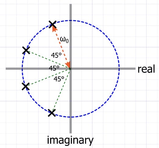
An s-plane representation of the transfer function of a fourth-order Butterworth filter.
Further Reading
In this article, we reviewed how the Laplace transform can help us extend our analysis of AC circuits with phasors to incorporate damped and steady-state sinusoids. To brush up on some other basics, like those involving transfer functions and phase shift in analog circuits, check out the articles below.
Understanding Poles and Zeros in Transfer Functions


The symbolic (s-domain) transfer function of linear active circuits can be found using nullor analysis. I posted an example for a Sallen-Key filter here:
https://www.mathworks.com/matlabcentral/fileexchange/73572-symbolic-analysis-of-an-active-linear-circuit-using-nullors
This simple example uses an ideal op-amp but you can use any linear circuit model, such as dominant pole. This example is matrix-based, which makes the approach systematic. You can continue onward with this approach and do other useful things like finding/plotting the change in the frequency response due to inexact component values (i.e., sensitivity analysis).