Gain Definitions for the Y-Factor Method of NF Measurements: Available Gain or Insertion Gain?

In principle, the Y-factor method is a relatively straightforward method of measuring the gain and noise figure (NF) of an RF component. However, there are some intricacies that require careful attention in practice. Several non-ideal effects, such as the uncertainty of the test equipment’s NF as well as the uncertainty related to the noise source itself, can lead to measurement uncertainty. Another subtlety is that the method actually measures and uses the DUT (device under test) insertion gain rather than its available gain.

 

Introducing the Y-Factor Method

The Y-factor method for noise figure measurement consists of two steps:

1. The measurement step shown in Figure 1(a) that determines the noise temperature of the DUT-Receiver system denoted by T_cas 
2. The calibration step of Figure 1(b) that determines the noise temperature of the receiver T_Receiver

 

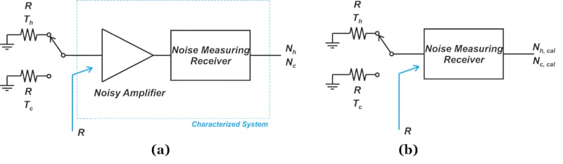
Figure 1. Two steps of Y-factor method for noise figure measurement: (a) measurement and (b) calibration

 

After measuring T_cas and T_Receiver, we can apply Friis’s equation to find the noise temperature of the DUT:

\[T_{cas} = T_{DUT} + \frac{T_{Receiver}}{G_{DUT}}\]

Equation 1.

 

where T_DUT and G_DUT denote the DUT’s noise temperature and gain, respectively. The noise powers obtained from the measurement setup (N_h and N_c in Figure 1(a)) are amplified by the DUT gain; however, N_h,cal and N_c,cal don’t experience this gain (Figure 1(b)). Therefore, G_DUT can be estimated by the following equation: 

\[G_{DUT} = \frac{N_h - N_c}{N_{h,cal}-N_{c,cal}}\]

Equation 2.

 

Available Power Gain

The power gain used in the noise figure definition is the available power gain,G_A, which is defined in the illustration of Figure 2 below. The available power gain is the ratio of the power available from the two-port network P_AVN (Figure 2(a)) to the power available from the source P_AVS (Figure 2(b)).

 

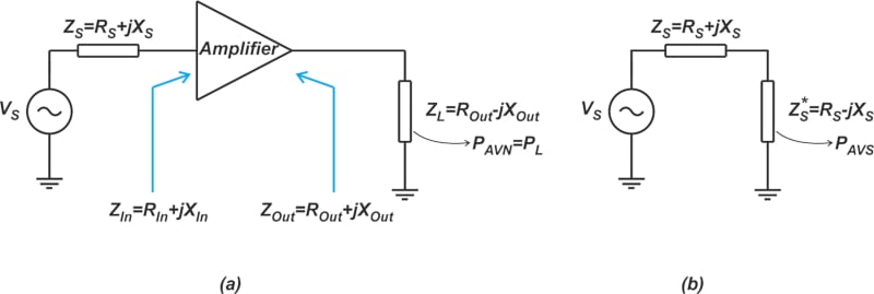
Figure 2. Available power gain definition

 

Note that for both P_AVN and P_AVS measurements, the measured port is connected to its conjugately-matched load. For example, to find P_AVN, the module output is connected to the complex conjugate of Z_out=R_out+jX_out, i.e. Z_L=R_out-jX_out. The power we obtain from Equation 1 is not the available power gain. To distinguish it from available gain, it is given a specific name: the insertion gain, which will be discussed below.

 

Insertion Power Gain

Figure 3 illustrates the definition of the insertion power gain.

 

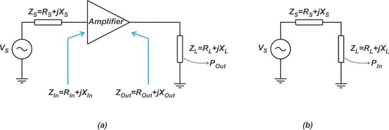
Figure 3. Insertion power gain definition

 

The insertion power gain depends on both source and load impedances (Z_S and Z_L). As shown in Figure 3(a), we connect the DUT to Z_L while its input is driven by a source impedance of Z_S, and measure the power delivered to the load (denoted by P_Out in Figure 3). We also measure the power that the source can directly deliver to Z_L, denoted by P_In in Figure 3(b). The ratio of P_Out to P_In is the insertion gain of the DUT. From this explanation, it should be clear that the insertion gain corresponds to the change in power gain that we obtain when we insert the DUT between a given Z_S and Z_L.    

 

Error Introduced by the Use of the Insertion Gain

Comparing the measurement and calibration steps of the Y-factor method (Figure 1(a) and (b)) with the insertion gain definition (Figure 3(a) and (b)), we observe that the gain we obtain from Equation 2 is actually the insertion gain rather than the available gain. It is possible to measure the DUT’s available gain; however, this requires two additional power measurements where the load impedance must be tuned to be a conjugate match to the port being measured.

The insertion gain, however, is obtained from the four power measurements required for the Y-factor method. We’re actually assuming that the insertion gain is equal to the available gain. If this is not the case, an error will be introduced in our measurements (Equation 1). It can be shown that the difference between the available gain G_A and insertion gain G_i is given by:

 

\[G_A (dB) - G_i (dB) = 10 log \Big ( \frac{(1-|\Gamma_s|^2)|1- \Gamma_1 \Gamma_2|^2}{(1-|\Gamma_2|^2)|1- \Gamma_1 \Gamma_s|^2} \Big )\]

Equation 3.

 

where Γ₁ is the reflection coefficient looking into the noise measuring receiver; Γ₂ is that observed looking into the output of the DUT; and Γ_s is the reflection coefficient of the noise source (Figure 4).  

 

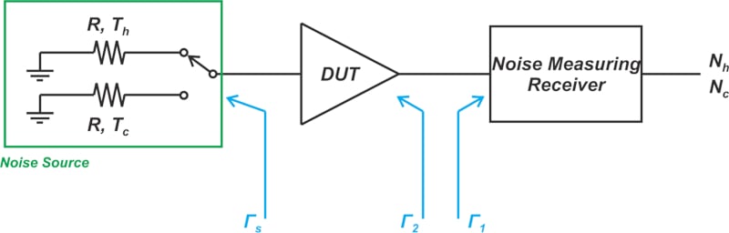
Figure 4. Reflection coefficients for the noise source, DUT output, and noise measuring receiver

 

Note that in the case of a perfect match (Γ₁=Γ₂=Γ_s=0), the insertion gain is equal to the available gain. In the above equation, knowledge of both the magnitude and phase of reflection coefficients is required to find G_A from G_i. Normally, the phase information is not available, and we can only find the error limits. Figure 5 shows the difference between the insertion gain and available gain as a function of match levels.

 

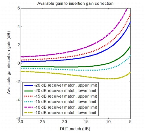
Figure 4. Ratio of available gain to insertion gain as a function of receiver and DUT matching. Image used courtesy of Anritsu.

 

In the above figure, the x-axis is the DUT input and output match (for simplicity, it’s assumed that the DUT’s input and output match are the same). The y-axis is the difference between the two power gains in decibels. The noise source match is assumed to be -20 dB, and the DUT is assumed to have decent isolation (|S21 × S12|= 0.1). Note that as the DUT match degrades beyond -10 dB, the difference between the two types of gain becomes more significant. In such cases, the gain error can introduce a significant error in the measured NF value.

 

S-Parameter Correction of Gain Error

At this point, you might wonder whether it is possible to use the S parameters of the DUT along with Equation 3 to obtain the available gain from insertion gain. By substituting G_A (rather than G_i ) into Friis’s equation, we can correct for the gain error. This appears to be of benefit, but there are two points that are worth mentioning.

First, note that we usually don’t have the phase information of the reflection coefficients (Γ₁, Γ₂, and Γ_s). With scalar measurements, we don’t know how the vector reflection coefficients will combine to produce the final error. Assuming that vector mismatches are available, we can find G_A from G_i.

However, there is another issue that can prevent us from having a more accurate measurement: the noise figure of the DUT and the measuring equipment is a function of their driving-point impedances. Figure 5 illustrates this graphically through the noise performance of a hypothetical DUT.

 

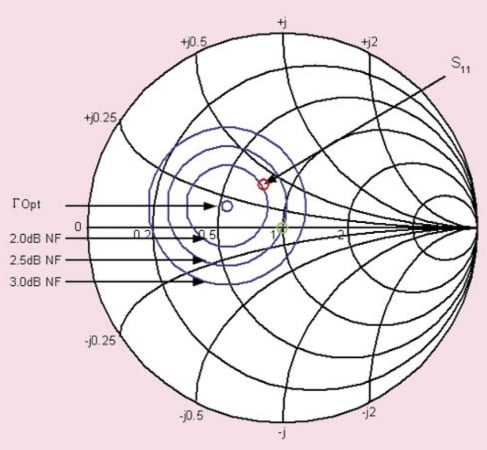
Figure 5. Smith Chart demonstrating impact of driving-point impedance on the noise figure. Image used courtesy of D. Boyd.

 

When the DUT is driven by a source impedance of 50 Ω (corresponding to the green circle at the center of the Smith chart), its noise figure is 2.5 dB. However, with a source impedance equal to the complex conjugate of the DUT’s S₁₁ (marked by the red circle in the figure), the noise figure is 2 dB. S parameters do not provide us with any information about the noise performance of the device. Therefore, while S parameter corrections can be used to find G_A from G_i, it won’t allow us to account for the change in the DUT’s NF. Without knowledge of the NF variation with source resistance, the S parameter correction can even increase the NF measurement error. 

Determining the NF dependence on the source impedance requires specialized NF measurement equipment that uses stub tuners to apply a range of complex impedances to the device. These measurements are then analyzed to produce the circular contours of NF on the Smith chart similar to that shown in Figure 5. It should be noted that common noise figure analyzers and network analyzers are not capable of producing these NF contours.

 

The Necessity of Specifying Measurement Uncertainty

Without having the noise contours, it is invalid to apply mismatch corrections for noise figure measurements. In these cases, it is recommended to minimize impedance mismatches of different ports as much as possible and then treat the residual mismatch as a measurement uncertainty. In addition to the mismatch effect, a complete uncertainty analysis can account for other non-ideal effects, such as the uncertainty of the test equipment’s NF as well as the uncertainty related to the noise source itself. Uncertainty analysis is key in every kind of measurement, including NF measurements. The following table highlights the importance of knowing measurement uncertainty by comparing two different hypothetical amplifiers.

 

	Noise Figure (dB)	NF Uncertainty (dB)
Amplifier 1	1.2	±0.5
Amplifier 2	1.4	±0.1

 

Without taking the uncertainty into account, one immediately chooses Amplifier 1 as the higher-performing device. However, considering the measurement uncertainty, we observe that Amplifier 1 can have a noise figure as large as 1.7 dB while the maximum NF of Amplifier 2 is 1.5 dB. When making noise figure measurements, a key parameter to be aware of is measurement uncertainty. In a future article, we’ll take a look at the measurement uncertainty of the Y-factor method.

 

Y-Factor Method Review

The Y-factor method actually measures and uses the DUT’s insertion gain rather than its available gain. This can lead to a significant error in the presence of impedance mismatches. Since the measurement of insertion gain is much easier than the available gain, we usually assume that these two power quantities are equal. To limit the error, however, impedance mismatches of different ports should be minimized. The residual mismatch error is usually treated as a measurement uncertainty.

 

Featured image used courtesy of Adobe Stock