Fourier Series Circuit Analysis—An Intro to Fourier Series Representation
Learn about the importance of the Fourier series in circuit analysis and the Fourier series equations, while gaining insight into how this analysis tool works.
The Fourier series is a powerful tool that enables expressing a non-sinusoidal periodic waveform as a sum of sinusoidal waveforms. In this article, we’ll first discuss the importance of the Fourier series by introducing one of its many applications, circuit analysis. Then, we’ll go over the Fourier series equations and attempt to develop some insight into how this analysis tool works.
Circuit Analysis Using a Sinusoidal Waveform: An RL Circuit Example
Before getting too far, it should be noted that sinusoidal waveforms play a key role in solving many engineering and scientific problems. For example, in circuit analysis, knowing the response to sinusoidal waveforms at different frequencies allows us to determine the steady-state response to other types of waveforms. To better understand this property, let’s examine the simple RL (resistor–inductor) circuit shown in Figure 1.
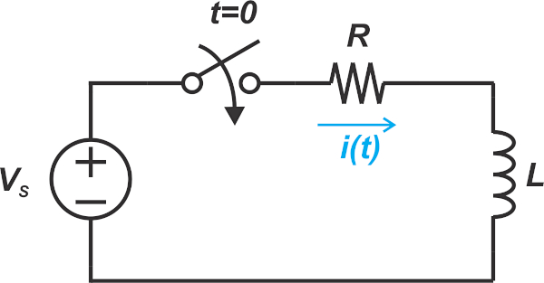
Figure 1. An example RL circuit.
Assume that the input is a sinusoidal voltage given by:
\[v_s = V_{m}cos(\omega t)\]
At t = 0, the switch is closed, and the input is applied to the circuit. It can be shown that the current flowing through the circuit is given by:
\[i=\frac{-V_{m}}{\sqrt{R^2+\omega^{2}L^{2}}}cos(\theta)e^{-(\frac{R}{L})t}+\frac{V_{m}}{\sqrt{R^2+\omega^{2}L^{2}}}cos(\omega t-\theta)\]
Where θ is a parameter that depends on ω, L, and R, and the first term in the above equation is the transient response of the system. As the name suggests, the transient response is temporary and typically quickly dies out with time, perhaps in a couple of milliseconds. If we keep the switch closed for a sufficiently long time, we’ll be left only with the second term, known as the steady-state response of the system.
The steady-state response is a sinusoidal wave at the same frequency as the input. Its phase and amplitude can differ from the input, however, it has the same shape and frequency. While we examined an RL circuit above, this property holds true for any other linear time-invariant (LTI) system, whether it's a complicated amplifier or a length of wire. If a circuit component is linear and time-invariant, its steady-state response to a sinusoidal input at frequency ω is a sinusoidal wave at the same frequency. This is not the case with other waveforms (e.g. a square wave), wherein the circuit can change the waveform shape and modify its amplitude and phase.
Steady-state Response to Sum of Two Sinusoidal Components
In the above example, we observe that the circuit changes the input phase by -θ and multiplies the input amplitude by the factor H given by:
\[H=\frac{1}{\sqrt{R^{2}+\omega^{2}L^{2}}}\]
This means that, by having θ and H, we can determine the steady-state response for a sinusoidal input at any arbitrary frequency ω. What if we simultaneously apply two sinusoidal inputs at ω1 and ω2? In other words, how will the circuit respond to the following input:
\[v_s = V_{m1}cos(\omega_{1} t) + V_{m2}cos(\omega_{2} t)\]
Since the circuit is assumed to be linear, the superposition principle states that the overall output is equal to the sum of the outputs produced by the individual input components. Therefore, the steady-state response is:
\[i=\frac{V_{m1}}{\sqrt{R^2+\omega_{1}^{2}L^{2}}}cos(\omega_{1} t-\theta_{1}) + \frac{V_{m2}}{\sqrt{R^2+\omega_{2}^{2}L^{2}}}cos(\omega_{2} t-\theta_{2})\]
Where θ1 and θ2 are the phase shifts experienced by the input components at ω1 and ω2, respectively. Therefore, if we know the response for sinusoidal components at different frequencies, we can determine the response to a sum of arbitrary sinusoidal components as well.
Steady-state Response to an Arbitrary Waveform
Let’s go one step further! Knowing the response to different sinusoidal inputs, can we determine the steady-state response to a periodic non-sinusoidal waveform? For example, if we input the square wave depicted in Figure 2, how can we determine the circuit’s steady-state response?
Note that Figure 2 shows only one period of the input waveform; in other words, the portion depicted in the figure is assumed to repeat itself in a periodic fashion over time.
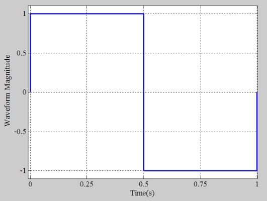
Figure 2. An example square wave.
This is where the Fourier series stands out. The Fourier series allows us to describe an arbitrary periodic waveform, such as the above square wave, in terms of sinusoidal waveforms. Since we know the circuit’s response to the individual sinusoidal components, we can also apply the superposition theorem to find the response to the arbitrary waveform.
Sum of Sinusoidal Functions: Learning From Sine Waves and Square Waves
Before going over the Fourier series equations, let’s try to paint a qualitative picture of how the sum of some sinusoidal functions can represent an arbitrary waveform. Consider the above square wave from Figure 2. Can we approximate this waveform by a single sinusoidal function?
As shown in Figure 3, a sine wave at the same frequency as the square wave (1 Hz in this example) fits nicely inside the square wave and exhibits identical zero-crossings along the x-axis. For the time being, let’s not worry about how the amplitude of this sine wave is chosen.
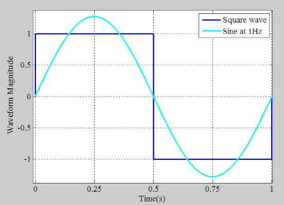
Figure 3. Approximating a square wave with a single sine wave.
In the above figure, the overall shape of the two waveforms has some similarities, but they are still very different. The square wave remains constant at each half-cycle. However, the sine wave reaches its maximum and minimum values at the midpoint of the positive and negative half-cycles of the square wave, respectively. Unlike the sine wave, the square wave changes more abruptly at the transitions.
Overall, it seems that the sine wave cannot catch up with the abrupt changes of the square wave. In that case, a single sine wave doesn’t seem to be an acceptable approximation of the square wave. However, what if we add another sinusoidal component? By adding another sine wave with appropriate amplitude and frequency, we might be able to achieve a better approximation. As shown by the red curve in Figure 4, this new sine wave is at 3 Hz in this example.
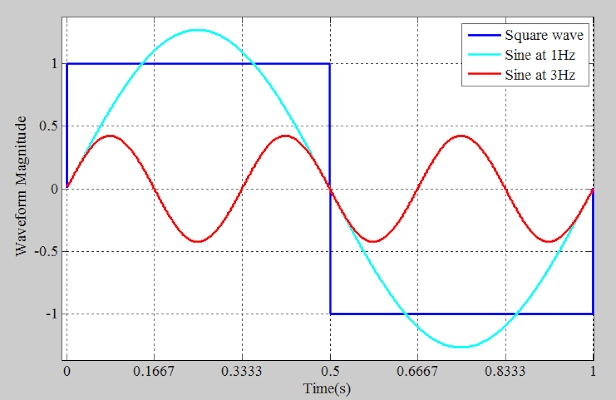
Figure 4. Example sine wave at 3 Hz.
The cyan and red curves have the same polarity in the vicinity of the square wave transitions. Therefore, when the two sine waves are added together, a waveform with transitions sharper than that of a single sine wave is created. However, for 0.1667 < t < 0.3333 and 0.6667 < t < 0.8333, the two sine waves have opposite polarity. With sharper transitions and flattened peaks and troughs, the sum of the two sine waves can produce a more accurate representation (Figure 5).
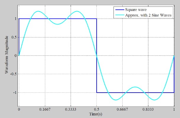
Figure 5. Example waveform of two sine waves and a square wave.
This suggests that, by adding more sinusoidal components with appropriate amplitude and frequency, we might achieve a better approximation of the square wave. For example, with 10 appropriately chosen sine waves, we get the waveform shown in Figure 6.
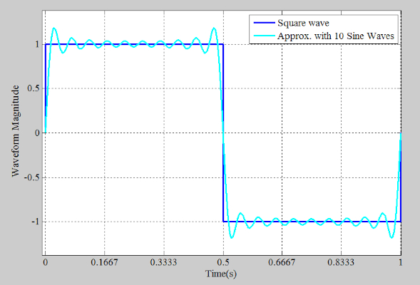
Figure 6. Example showing a square wave and 10 sine waves.
Now that we know it is possible to represent a periodic signal as the sum of sinusoidal components, the remaining question is, how are these sinusoidal components calculated for a given waveform?
Understanding the Fourier Series Equation—Finding the Fourier Series Representation
Assume that f(t) is a periodic signal with period T. We can express f(t) in terms of an infinite sum of sinusoidal components as follows:
\[f(t)=a_0 + \sum_{n=1}^{\infty}a_{n}cos(n\omega_{0}t)+\sum_{n=1}^{\infty}b_{n}sin(n\omega_{0}t)\]
Equation 1.
Where:
- a0, an, and bn are the Fourier coefficients of the signal
- \(\omega_{0}=\frac{2\pi}{T}\) represents the fundamental frequency of the periodic signal
The frequency \(n\omega_{0}\) is known as the n-th harmonic of the waveform. The coefficients can be calculated by the following equations:
\[a_0 = \frac{1}{T}\int_{-\frac{T}{2}}^{+\frac{T}{2}}f(t)dt\]
Equation 2.
\[a_n = \frac{2}{T}\int_{-\frac{T}{2}}^{+\frac{T}{2}}f(t)cos(n \omega_0 t)dt\]
Equation 3.
\[b_n = \frac{2}{T}\int_{-\frac{T}{2}}^{+\frac{T}{2}}f(t)sin(n \omega_0 t)dt\]
Equation 4.
Note that the integrals can be taken over any arbitrary period of the waveform, meaning that it doesn’t necessarily need to be the $$-\frac{T}{2}$$ to $$+\frac{T}{2}$$ interval.
However, it needs to be one full period of the waveform. Appropriately choosing the starting point of the integral can make the calculations less cumbersome in some cases.
For example, let's find the Fourier series for the periodic voltage shown in Figure 7.
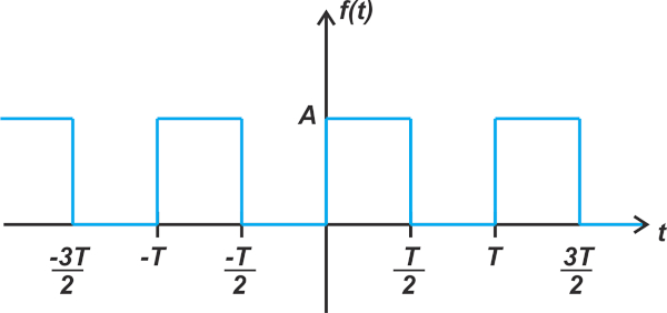
Figure 7. Example of periodic voltage.
By applying Equation 2, we obtain:
\[a_0 = \frac{1}{T}\int_{-\frac{T}{2}}^{+\frac{T}{2}}f(t)dt=\frac{1}{T}\int_{-\frac{T}{2}}^{0}0 \times dt + \frac{1}{T}\int_{0}^{\frac{T}{2}}A \times dt=\frac{A}{2}\]
Next, Equation 3 yields the an coefficients as:
\[a_n = \frac{2}{T}\int_{-\frac{T}{2}}^{+\frac{T}{2}}f(t)cos(n \omega_0 t)dt=\frac{2}{T}\int_{0}^{+\frac{T}{2}}Acos(n \omega_0 t)dt = 0\]
If you read my other article in this series, which is on the symmetry of the Fourier coefficients, the above result should be no surprise. After eliminating the DC value of the square wave in Figure 7, we obtain a waveform with odd symmetry. For an odd signal, we have an = 0 for all n.
Finally, by applying Equation 4, we obtain the bn coefficients as follows:
\[b_n = \frac{2}{T}\int_{-\frac{T}{2}}^{+\frac{T}{2}}f(t)sin(n \omega_0 t)dt=\frac{2}{T}\int_{0}^{+\frac{T}{2}}Asin(n \omega_0 t)dt\]
You can verify that the above integral works out to zero for even n. For odd values of n, we obtain:
\[b_n = \frac{2A}{n \pi}\]
Therefore, substituting our findings into Equation 1, we can write the Fourier series of this waveform as:
\[f(t)=\frac{A}{2} +\frac{2A}{\pi}\sum_{n=1}^{\infty}\frac{sin((2n-1)\omega_{0}t)}{2n-1}\]
Please note how the n variable is adjusted to consider that only sinusoids at odd multiples of \(\omega_{0}\) are non-zero.
Fourier Analysis—a Versatile Tool in Circuit Analysis
Although we introduced the Fourier series starting with its application in circuit analysis, it should be noted that the Fourier series and its variants are also widely used for other purposes. For example, an important tool closely related to the Fourier series is the discrete Fourier transform (DFT), whose computationally-efficient implementation is known as the fast Fourier transform (FFT). The FFT is used in radar applications to determine the distance and velocity of a target, among its numerous other applications.
Interestingly, Fourier analysis is also a truly ubiquitous tool in nature—so much so that some people describe it as nature's way of analyzing data. According to Peter Moore, a Yale professor of biophysics, our eyes and ears subconsciously perform the Fourier transform to interpret sound and light waves.
The Fourier series discussed above allows us to decompose a signal to its constituent sinusoidal components at different frequencies. This enables us to determine how the signal power is distributed in the frequency domain.
The Fourier series is used to analyze periodic waveforms. For an aperiodic waveform, a generalization of the Fourier series, known as the Fourier transform, should be used.
For all signals of practical interest, the Fourier series exists, meaning that the sum of the sinusoidal components converges to the original waveform. However, from a mathematical point of view, we might not be able to express a given periodic function as a convergent Fourier series. The requirements sufficient to assure convergence are known as the Dirichlet conditions. This limitation, however, does not present a serious problem in practice because the Dirichlet conditions are satisfied by the waveforms generated in physical systems.
Featured image used courtesy of Pixabay
To see a complete list of my articles, please visit this page.