Technical Article

Understanding RF Power Measurement Errors in Directional Couplers

January 31, 2024 by Dr. Steve Arar

Directional couplers are valuable tools for testing RF systems. However, the finite directivity of these devices can cause measurement uncertainty. Learn more in this article.

Directional couplers play a fundamental role in many microwave and millimeter-wave systems. For example, vector network analyzers (VNAs) use directional couplers to separate and sample the forward and backward waves that travel to and from the DUT’s port. In this article, we’ll discuss how the directivity factor of a coupler can introduce error when measuring reflected power.

Measuring Reflected Power

Figure 1 illustrates a generic directional coupler measuring the power reflected from an unknown termination. Because we’re measuring reflected power, the load side of the coupler (Port 1) is labeled as the input port, even though the source is connected to Port 2.

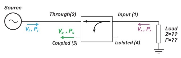
Using a directional coupler to measure reflected power. All four ports are shown, though the isolated port is terminated.

Figure 1. Using a four-port directional coupler to measure reflected power. Image used courtesy of Steve Arar

The power applied by the source (P_i) passes through the coupler to the load—from Port 2 to Port 1. At the load, a portion of the power is reflected back toward the coupler. The amount of reflected power (P_r) is a function of the difference between the load impedance and the characteristic impedance of the interconnection. A small portion of P_r transfers through the coupler and exits through Port 3, the coupled port.

In an ideal world, knowing P_i and measuring the coupled power (P_c) would allow us to determine the load reflection coefficient (Γ). For example, if the load is perfectly matched, no power is reflected, and so P_c should ideally be zero.

However, a real-world directional coupler will leak a bit of P_i incident on Port 2 to the coupled Port 3, which affects power measurement accuracy. The amount of leakage depends on the coupler's directivity. In the rest of this article, we’ll examine how this error is quantified.

Review of Directional Coupler Equations

In the previous article in this series, we introduced the three factors commonly used to characterize directional couplers:

Coupling factor (C).
Directivity factor (D).
Isolation factor (I).

For the four-port directional coupler in Figure 1, we can calculate these quantities as follows:

$$ C \text{ (dB)}~=~10 \times \log \left( \frac{P_1}{P_3} \right) ~=~ P_1 \text{ (dB)} ~-~ P_3 \text{ (dB)} $$

Equation 1.

$$ D \text{ (dB)} ~=~ 10 \times \log \left( \frac{P_3}{P_4} \right) ~=~ P_3 \text{ (dB)} ~-~ P_4 \text{ (dB)} $$

Equation 2.

$$I \text{ (dB)} ~=~ 10 \times \log \left( \frac{P_1}{P_4} \right) ~=~ P_1 \text{ (dB)} ~-~ P_4 \text{ (dB)} $$

Equation 3.

where:

P_x is the power at Port x in watts.

P_x (dB) is the power at Port x in dB.

There’s an interesting relationship between the three factors:

$$I ~=~ P_1 ~-~ P_4 ~=~ (P_1 ~-~ P_3) ~+~ (P_3 ~-~ P_4) ~=~ C ~+~ D$$

Equation 4.

Calculating the Reflected Power at the Coupled Port

To begin with, we’ll calculate the ideal power that reaches the coupled Port 3. Let’s assume that all of the power from the source (P_i) and incident on Port 2 passes out of Port 1. The power in dB reflected from the load (P_r) is then equal to the incident power (P_i) minus the load’s return loss (RL):

$$P_r ~=~ P_i ~-~ RL$$

Equation 5.

A fraction of the input power on Port 1 is coupled to Port 3. By rearranging Equation 2, we can represent the coupled power out of Port 3 by:

$$ P_3 ~=~ P_1 ~-~ C $$

Equation 6.

We’ll refer to this coupled power out of Port 3 as P_c₁. Now, by substituting P_r for P₁, we get:

$$ P_{c1} ~=~ P_r ~-~ C $$

Equation 7.

Finally, substituting Equation 5 into Equation 7, we have:

$$P_{c1} ~=~ P_i ~-~ RL ~-~ C$$

Equation 8.

Figure 2 illustrates the relationship between the power terms, the coupling factor, and the return loss.

Relationship between power terms, coupling factor, and return loss for a directional coupler.

Figure 2. Relationship between the power terms, coupling factor, and return loss. Image used courtesy of Steve Arar

Multiple Reflections Make Things More Difficult!

In this analysis, we assumed that the power reflected from the load and passed back through the coupler is fully absorbed by the input port of the coupler (Port 1). In practice, this port might not be perfectly matched. Consequently, multiple reflections can occur between the coupler and the load, further changing the measurement error.

Calculating the Power Measurement Error Caused by Finite Directivity

Now we need to start thinking about the sources of error in the coupler. Since the coupler has finite directivity, a small fraction of P_i also leaks to Port 3. We’ll call this leakage P_c₂.

For a wave incident on Port 2, Port 3 is the isolated port. Therefore, the amount of leakage is characterized by the isolation factor with a slightly different equation:

$$ I \text{ (dB)} ~=~ P_2 \text{ (dB)} ~-~ P_3 \text{ (dB)} ~=~ P_i ~-~ P_{c2}$$

Equation 9.

Rearranging this equation and substituting from Equation 4, we get:

$$ P_{c2} ~=~ P_i ~-~ I ~=~ P_i ~-~ (C ~+~ D) $$

Equation 10.

This set of relationships is shown in Figure 3. P_c₁ is the desired signal that specifies the return loss of the load, and P_c₂ is the signal that leaks from Port 2 to Port 3.

Relationship of coupled power and leakage power in reflected power measurement.

Figure 3. Relationship of coupled oiwer and leakage power in reflected power measurement. Image used courtesy of Steve Arar

P_c₂ is only present because of the finite directivity of the coupler. Ideally, the directivity (D) would be infinite, and the measured power would be a function only of the power reflected from the load. When D is finite, an additional power term (P_c₂) appears at the coupled port, affecting our measurement accuracy.

As we can see in Figure 3, the difference between P_c₁ and P_c₂ is equal to D – RL. Given the directivity and return loss, we can easily determine how small P_c₂ is relative to the desired power. For example, if D = 34 dB and RL = 26 dB, we know that P_c₂ is 8 dB lower than P_c₁.

Accounting for the Phase Difference

Above, we determined the relationship between the desired power measurement (P_c₁) and the undesired leakage (P_c₂). However, the overall power measured at the coupled port also depends on the phase difference between these two signal components.

Let’s assume that the voltage signals corresponding to P_c₁ and P_c₂ are sinusoidal waveforms with amplitudes a and b, respectively. Using the relationships demonstrated in Figure 3, we have:

$$a~=~10^{-(C+RL)/20}~\times~V_{i}$$

Equation 11.

and:

$$b ~=~ 10^{-(C+D)/20} ~\times~ V_{i}$$

Equation 12.

where V_i is the amplitude of the incident voltage from the source in Figure 1.

If the two signals are in phase, the overall signal amplitude will be a + b. On the other hand, if the two signals are 180 degrees out of phase, the overall amplitude will be a – b. These two extreme cases give the maximum and minimum of the overall signal—other values of the phase difference produce an amplitude between a – b and a + b.

The overall voltage wave at the coupled port can be expressed as:

$$\begin{eqnarray} V_{c} ~&=&~ a ~+~ b ~\times~ e^{j \theta} \\ &=&~ 10^{-(C+RL)/20} ~\times~ V_{i} ~\times~ \big (1~+~10^{(RL-D)/20} e^{j \theta} \big ) \end{eqnarray}$$

Equation 13.

The terms in Equation 13 can be understood as follows:

The term e^jθ accounts for the phase difference between the two signals.
The term inside the parentheses is the error factor that characterizes the relative deviation of the measurement from the actual value.
The terms in front of the parentheses represent the desired amplitude that we would get if the coupler had infinite directivity.

We’ll call this desired amplitude V_desired, and write out its equation separately:

$$ V_{desired} ~=~ 10^{-(C+RL)/20} ~\times~ V_{i} $$

Equation 14.

We can then rewrite Equation 13 as:

$$V_{c} ~=~ V_{desired} ~\times~ (1~+~x ~\times~ e^{j \theta})$$

Equation 15.

where x is equal to 10^{(RL – D)/20}. The overall error factor is a vectorial summation of 1 and x. Figure 4 helps us visualize the error term.

The error factor, visualized as a vector with real and imaginary parts.

Figure 4. Visualizing the error factor as a vector with real and imaginary parts. Image used courtesy of Steve Arar

Example 1: Calculating the Uncertainty of Measured Return Loss

To clarify the above discussion, let’s solve an example problem from Rohde & Schwarz’s document on VNA fundamentals. In this example, we aim to measure a load with an actual return loss (RL) of 30 dB, using a coupler with a directivity (D) of 40 dB. What are the maximum and minimum values of the measured return loss?

From Figure 3, we know that the difference between the desired signal power and the undesired signal power is equal to D – RL = 40 - 30 = 10 dB. Therefore, the amplitude of the undesired voltage is a factor of 0.32 less than the desired voltage, as calculated below:

$$x~=~10^{(RL-D)/20}~=~10^{-10/20}~=~0.32$$

Equation 16.

Plugging this value of x into Equation 15, we see that the overall voltage can be either:

A factor of 1 + x = 1.32 higher than the actual value.
A factor of 1 – x = 0.68 lower than actual value.

Therefore, the measured power can be:

20log(1.32) = 2.4 dB higher than the actual value.
20log(0.68) = 3.35 dB lower than the actual value.

The measured reflected power is related to the return loss of the load. A higher reflected power corresponds to a smaller return loss. When the measured reflected power is 2.4 dB higher than the actual value, the measured return loss is 2.4 dB lower than its actual value. This leads to:

$$RL_{measured} ~=~ RL_{actual} ~-~ 2.4 ~=~ 30 ~-~ 2.4 ~=~ 27.6 \text{ dB}$$

Equation 17.

Similarly, when the measured reflected power is 3.35 dB lower than the actual value, the measured return loss is 30 + 3.35 = 33.35 dB. The measured return loss can therefore be anywhere between 27.6 dB and 33.35 dB.

Example 2: Calculating the Uncertainty of Measured Return Loss

To get more comfortable with these calculations, let’s take a look at another example. Assume that we aim to use a directional coupler with directivity of 35 dB to measure a load with an actual return loss of 20 dB. Following a procedure similar to the above example, we first find how small the amplitude of the undesired voltage is relative to the desired voltage:

$$x~=~10^{(RL-D)/20}~=~10^{(20-35)/20}~=~0.18$$

Equation 18.

The overall voltage can be either:

A factor of 1 + 0.18 = 1.18 higher than the actual value.
A factor of 1 – 0.18 = 0.82 lower than the actual value.

Therefore, the measured power can be either:

20log(1.18) = 1.44 dB higher than the actual value.
20log(0.82) = 1.72 dB lower than the actual value.

When the measured reflected power is 1.44 dB higher than the actual value, the measured return loss is 20 – 1.44 = 18.56 dB. On the other hand, when the power is measured to be 1.72 dB lower, the measured return loss is 20 + 1.72 = 21.72 dB. Therefore, the measured return loss can be anywhere between 18.56 dB and 21.72 dB.

How Does the Error Change with Return Loss and Directivity?

Figure 5 plots the error in measuring the reflected power for different values of return loss and directivity.

Reflected power measurement error as a function of return loss and directivity.

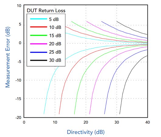
Figure 5. Reflected power measurement error as a function of return loss and directivity. Image used courtesy of Marki Microwave

The above plot corresponds to a coupler with a 1 dB insertion loss. This makes the results slightly different from those produced by our analysis, in which we ignored the coupler’s insertion loss. However, the plot reveals some important properties of the error introduced by finite directivity.

First, note that the error increases with the return loss. For a given input power (P_i), the leakage power is constant, but the measured signal (P_r) is decreasing.

Second, observe that increasing directivity for a given return loss reduces the error. The relationships in Figure 3 explain why: as we increase D, the undesired signal becomes smaller and smaller compared to the desired signal, improving the measurement accuracy.

Figure 5, which is taken from a Marki Microwave white paper titled “Directivity and VSWR Measurements: Understanding Return Loss Measurements,” shows how the error becomes excessively large when directivity is nearly equal to the load’s return loss. The white paper suggests, as a rule of thumb, that you can reduce the error to about 1 dB by using a directivity about 15 dB higher than the DUT return loss. For example, if the return loss is 20 dB, we would need a directivity of 35 dB to limit the error to 1 dB.

Measuring Forward Power

We can also use a directional coupler to sample the forward power, as Figure 6 illustrates.

Using a three-port directional coupler to sample the forward power.

Figure 6. Using a three-port coupler to sample the forward power. Image used courtesy of Steve Arar

Compared to reflected power measurement, the directivity requirement of the coupler for forward power measurement is more relaxed. This is because the input power (P_i) being measured is larger than the reflected power (P_r). Figure 7 shows the forward power measurement error for different return loss and directivity values.

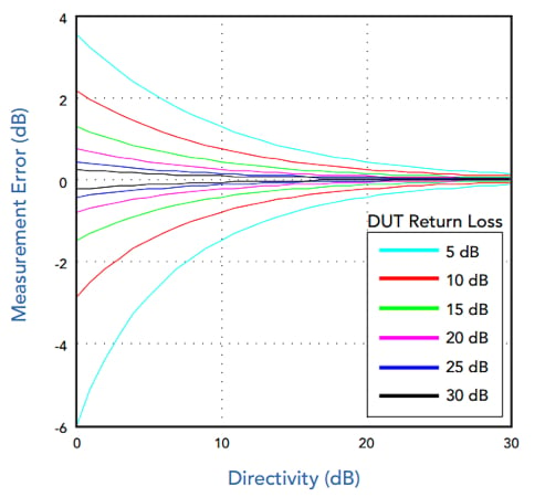
Forward power measurement error as a function of return loss and directivity.

Figure 7. Forward power measurement error as a function of return loss and directivity. Image used courtesy of Marki Microwave

Note that the error gets bigger when the load return loss is smaller. That’s because a lower return loss means that more power is reflected back to the source. That, in turn, causes the undesired signal at the coupler’s output to grow. Even for a very small return loss, though, a directivity of 15 dB can ensure that the error of the forward measurement doesn’t exceed approximately 1 dB.

Measuring Directivity of a Coupler

As a final note, since it’s closely related to the error analysis provided in this article, I’d like to mention a practical method for measuring the directivity of a coupler. We generally can’t measure this directivity directly, because the forward and backward waves produce comparable signal components at the coupler’s output.

However, we can modify Figure 1 to measure a coupler’s directivity indirectly using a sliding load, as shown in Figure 8.

Circuit for measuring the directivity of a coupler.

Figure 8. Circuit for measuring the directivity of a coupler. Image used courtesy of Steve Arar

Changing the position of the sliding load introduces a variable phase shift in the reflected signal. From our discussion above, we know that the voltage at the coupled port produces a circular contour (Figure 4) as we change the position of the sliding load. By finding the minimum and maximum power levels at the coupled port, we can determine the directivity of the coupler.

This article is Part 2 of a series on vector network analyzers. In order of publication, the articles in this series are: