How to Estimate and Enhance the Dynamic Range of a Vector Network Analyzer

As we learned in a previous article, the dynamic range of a vector network analyzer (VNA) plays a key role when measuring, for example, the frequency response of a highly selective filter. In this article, we’ll learn how to estimate the VNA dynamic range you need for your measurements. We’ll also discuss four methods for improving VNA dynamic range, namely:

1. Signal averaging.
2. Adjusting the intermediate frequency (IF) bandwidth.
3. Segmented sweeps.
4. Using reconfigurable test ports.

Before we dive into our main topic, we’ll briefly review how a VNA’s dynamic range affects its ability to measure filter response accurately. Then, we’ll examine the inaccuracies that can result from interfering signals. Once we have that background information, we’ll be ready to discuss techniques that can help us avoid measurement error resulting from inadequate dynamic range.

 

Dynamic Range in Filter Response Measurement

The dynamic range of a system is defined as the difference between the highest- and lowest-amplitude signals that the system can measure, as illustrated in Figure 1.

 

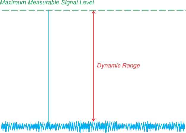
Figure 1. Demonstration of dynamic range. Image used courtesy of Steve Arar

 

Figure 2 demonstrates why the dynamic range of a VNA is a critical factor when measuring filters with large stop-band rejection.

 

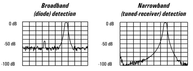
Figure 2. Frequency response of a band-pass filter measured using a VNA with poor dynamic range (left) and good dynamic range (right). Image used courtesy of Agilent Technologies

 

In the left-hand portion of Figure 2, a VNA with a sensitivity of about –60 dB is used to measure a filter that has 90 dB of stop-band rejection. The poor dynamic range results in VNA mostly measuring its own noise floor rather than the filter’s stop-band behavior. In the right half of the figure, the same filter is measured using a VNA with a sensitivity of –100 dBm. The increased dynamic range provides a more accurate measure of the filter response.

Now that we’ve reviewed the importance of dynamic range, let’s explore the effect of an interfering signal on our measurement.

 

Interfering Signals and Measurement Error

Let’s say that we intend to measure a single-tone input, and an undesired signal component shows up at our measured frequency spectrum. For the purpose of discussion, we’ll assume two signals at the same frequency:

• The desired signal has an amplitude of 1.
• The undesired signal has an amplitude of x, where x is much less than 1.

The overall measured amplitude (V_m) can be written as the sum of these two components:

$$V_{m} ~=~ 1~+~x ~\times~ e^{j \theta}$$

Equation 1.

 

In the above equation, the term e^jθ is included to account for the arbitrary phase difference (θ) between the two signals. The overall signal is a vectorial summation of 1 and x; the measured value depends on the phase difference between the two signals. Figure 3 can help us visualize how the undesired component affects our measurement as θ changes.

 

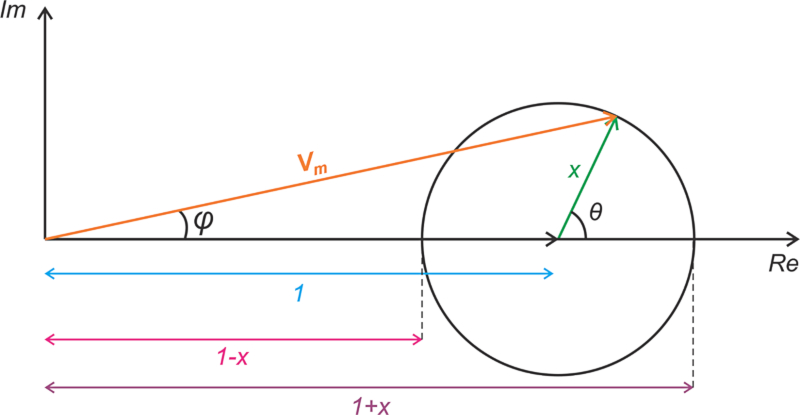
Figure 3. Vector representation of the desired and undesired signals. Image used courtesy of Steve Arar

 

Depending on θ, the magnitude of the measured value can be anywhere between 1 – x and 1 + x. The ratio of V_m to the desired amplitude (unity) is the magnitude measurement error. Therefore, expressed in decibels, the magnitude error can span from 20log(1 – x) to 20log(1 + x). These two error limits (positive magnitude and negative magnitude) are plotted in Figure 4 along with the phase error.

 

Figure 4. Measurement error as a function of interfering signal amplitude and phase. Image (modified) used courtesy of Agilent Technologies

 

For example, let’s say that the amplitude of the undesired signal is x = 0.1, which corresponds to an interfering signal amplitude 20 dB below the desired signal. The error will be between –0.92 dB and 0.83 dB. We can also use the above error plot as a graphical tool to estimate the error, which leads to a similar value.

As we saw in Figure 3, the undesired signal also affects the phase angle of V_m. The phase error this produces has a maximum value of φ_max = arcsin(x). When x is 20 dB below the desired signal, we have φ_max = 5.74 degrees, which is consistent with the phase error curve provided in Figure 4.

 

Estimating the Required Dynamic Range: Method and Example

The question now arises: how much dynamic range should the VNA provide for a given measurement error? An exact answer to this question would require a complicated analysis. However, we can obtain a rough estimate of the required dynamic range by assuming that the VNA’s noise floor has the same amplitude as the undesired signal that’s interfering with our measurement.

To understand this technique, let’s use the error plot in Figure 4 to work through an example. This example, along with the math in the previous section, can also be found in an Agilent Technologies document titled “Agilent Network Analyzer Basics.”

Let’s say we want to measure the frequency response of a filter with 80 dB stop-band rejection. What VNA dynamic range do we need to keep the magnitude error of the measured response below 0.1 dB? Assume that only a single interfering signal is present.

We can see in Figure 4 that a magnitude error of no more than 0.1 dB corresponds to an interfering signal amplitude that’s about 39 dB below the desired signal amplitude. To achieve the required level of accuracy when measuring the stop-band of the filter, the noise floor of the VNA should therefore be 39 dB lower than the filter’s stop-band response. We also know that the filter’s stop-band attenuation is 80 dB more than its pass-band attenuation. The VNA should therefore provide a dynamic range of about 80 + 39 = 119 dB.

Some modern VNAs provide a dynamic range of 150 dB, but we can still consider the 119 dB dynamic range relatively high. These levels of dynamic range can be achieved by applying the signal averaging technique and/or adjusting the VNA’s intermediate frequency (IF) bandwidth, as we’ll discuss in subsequent sections of the article.

Before we move on, though, what would the phase error be if we keep the magnitude error below 0.1 dB? If we look back at Figure 4, we can see that a magnitude error of less than 0.1 dB corresponds to a phase measurement error of no more than 0.65 degrees.

 

Signal Averaging

In general, to reduce the effect of noise on our measurements, we can repeat the measurement multiple times and average the measured values. Since the noise samples aren’t correlated, signal averaging suppresses the noise terms without affecting the actual deterministic output of the circuit.

If we repeat the measurement M times, the signal averaging will reduce the original noise variance by a factor of M. Put differently, the signal-to-noise ratio (SNR) improves by 3 dB every time the average doubles.

Signal averaging is a powerful technique for lowering the noise floor of a VNA and improving its dynamic range, which is why most VNAs have an averaging function. Because it requires repeated measurements, however, averaging results in an overall increased measurement time.

For example, let’s consider what happens when we increase the averages from 10 to 100 for a given VNA IF bandwidth. Since the number of averages is increased by a factor of 10, we know that the noise variance (or the noise average power) reduces by a factor of 10. In terms of decibels, the SNR improves by 10log(10) = 10 dB. Put differently, the noise floor is reduced by 10 dB. Due to the increased number of measurements, however, the sweep time increases tenfold.

 

Adjusting the IF Bandwidth

VNAs allow us to adjust the bandwidth of the digital filters in the IF section of receivers. By making these filters narrower, we can remove a larger portion of the noise, thus improving the dynamic range of the filter. As with the averaging technique, however, this improvement is achieved at the cost of increased measurement time.

A VNA characterizes the DUT’s response by performing measurements at a certain number of frequency points across the specified frequency span. The per-point measurement time depends on the settling time of the IF filter. Copper Mountain Technologies provides the following equation for IF filter settling time:

$$\text{IF Filter Settling Time}~=~\frac{\text{IF Bandwidth Coefficient}}{\text{IF Bandwidth}}$$

Equation 2.

 

The IF bandwidth is given in Hz; the IF bandwidth coefficient varies by VNA model. Figure 5 shows how the IF bandwidth affects the dynamic range and the IF filter settling time of the SC5090 VNA. This VNA, like many others from Copper Mountain Technologies, has an IF bandwidth coefficient of 1.18.

 

Figure 5. Dynamic range and settling time versus IF bandwidth for an example VNA. Image used courtesy of Copper Mountain Technologies

 

Due to narrower IF filters requiring more time to settle, the measurement time is inversely proportional to the user-selectable IF bandwidth. For example, Equation 2 predicts that the IF filter settling time will be reduced by a factor of 10⁶ if we increase the IF bandwidth from 1 Hz to 1 MHz. This is consistent with data provided in Figure 5, which shows that the settling time falls from 1.18 seconds to 1.18 µs.

Because the noise power that enters the system is proportional to the system bandwidth, increasing the IF filter bandwidth from 1 Hz to 1 MHz also increases the noise power by a factor of 10⁶. In decibels, this corresponds to a noise floor increase of 10log(10⁶) = 60 dB. We can see in Figure 5 that this increase in bandwidth causes the VNA’s dynamic range to decrease by 60 dB (from 150 dB to 90 dB).

Compared to signal averaging, the IF bandwidth reduction method might provide a slightly faster measurement time for a given dynamic range improvement. If measurement speed is a critical factor in your application, you can refer to the Keysight application note “Understanding and Improving Network Analyzer Dynamic Range” for further details. If not, either method should work equally well.

 

Segmented Sweeps

We can also improve dynamic range by using a segmented, as opposed to linear, frequency sweep. This involves breaking up the frequency span of measurement into two or more segments. Each segment can have its own measurement parameters (number of frequency points, IF bandwidth, power level, etc.), allowing us to optimize the speed and dynamic range for each segment.

The segmented sweep method can be very helpful when characterizing highly selective filters. We can use a wide IF bandwidth in the pass-band of the filter, where noise might be of less concern, while also employing a low IF bandwidth in the stop-band of the filter, which can be highly affected by the noise.

 

Reconfigurable Test Ports

Some VNAs allow the user to achieve extremely high dynamic ranges by reconfiguring the test ports. In these models, the ports of the directional coupler within the VNA are routed to the front panel so that the user can modify the path by which the signal reaches the measurement receiver. Figure 6 shows a test port configuration that can be used to increase the dynamic range.

 

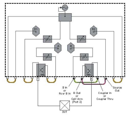
Figure 6. Configuration model of a VNA’s test ports. Image used courtesy of Keysight

 

In the above diagram:

• R1 and R2 are the reference receivers.
• A and B are the measurement receivers.

The left-hand test port is connected to the input port of the DUT. This test port has a standard connection. However, the other test port is configured to bypass the directional coupler.

The output of the DUT is connected to the measurement receiver path through the main line of the coupler. As a result, the coupler’s loss from the main line to the coupled port is no longer in the measurement path, as it was in the standard connection. Eliminating this loss term increases the effective sensitivity of the analyzer, usually by 14 dB or more.

With the above configuration, the coupler is no longer part of the signal path. Because of this, the VNA can’t be used to make reverse measurements. Also, note that power into the receiver must be monitored to prevent compression. We can then use the segmented sweep method to adjust the power level as needed. When measuring filters, for example, we can conduct a segmented sweep using higher power levels in the stop-band and lower power levels in the pass-band. +10 dBm in the stop-band and –6 dBm in the pass-band are typical choices here.

 

Wrapping Up

In this article, we learned about a simple method to estimate the dynamic range a VNA requires to take a given measurement, along with several methods for improving the dynamic range. Early on, we also explored the effect of interfering signals on measurement accuracy. We’ll return to this when, in future articles, we discuss how a VNA can be calibrated to reduce measurement uncertainty.

 

This article is Part 5 of a series on vector network analyzers. In order of publication, the articles in this series are:

1. Introduction to the Directional Coupler for RF Applications
2. Understanding RF Power Measurement Errors in Directional Couplers
3. Understanding the Inner Workings of Vector Network Analyzers
4. Understanding the Significance of Dynamic Range and Spurious-Free Dynamic Range
5. How to Estimate and Enhance the Dynamic Range of a Vector Network Analyzer
6. Introduction to VNA Calibration Techniques
7. Understanding the Limits of VNA Calibration
8. Understanding the 12-Term Error Model and SOLT Calibration Method for VNA Measurements
9. Understanding RF Calibration Using Short, Open, Load, and Through Terminations

 

Featured image used courtesy of Adobe Stock