
Noise Analysis Using LTspice Tutorial
Learn how to simulate noise using LTspice and use this great tool to learn more about low-noise design.
Learn how to simulate noise using LTspice and use this great tool to learn more about low-noise design.
One fascinating capability of LTspice is the ability to model noise in your circuit. This article covers the basics of performing a noise analysis and displaying the results, beyond basic circuit simulation with LTspice.
We assume you know how to create an LTspice schematic and run an AC analysis. If you don't know much about the theory of noise, use LTspice with the techniques presented here to help you learn. If you are familiar with noise, use this article to jump-start using this part of LTspice. There is even an undocumented bonus tip.
Modeling noise is a bit different from other modeling such as AC analysis. LTspice finds noise sources within individual components of your circuit; in other words, these noise sources are not specified with separate signal sources that are placed in the schematic. Noise analysis involves keeping track of individual noise sources and how these sources add together to produce a total output noise.
Having LTspice automatically do all the “bookkeeping” is a huge advantage over manual analysis. There are limitations to be discussed later, but let's get started on the basics.
Here are some LTspice noise simulation examples.
Simulation 1: A Resistive Voltage Divider
We start with a voltage divider used to establish a voltage reference or bias in a circuit with a single supply voltage. Resistors produce “thermal” noise, and the amount of noise depends on the value of the resistance, the bandwidth, and the temperature (we start with the default temperature).
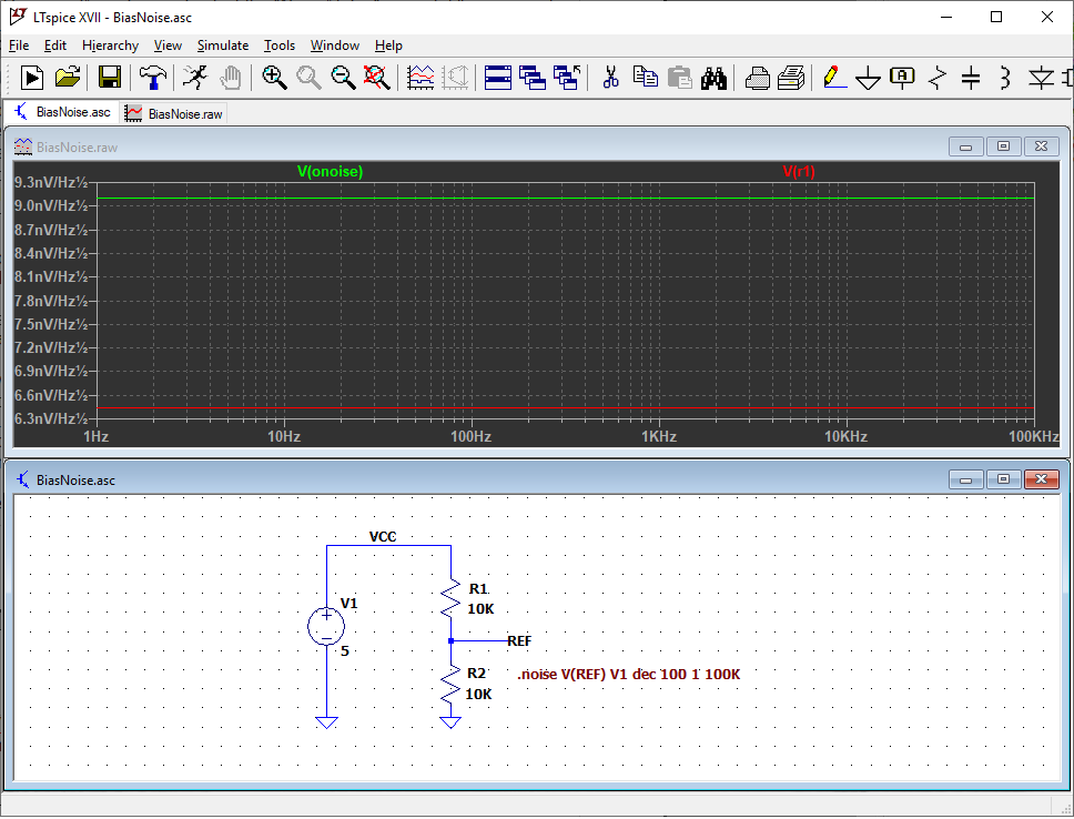
As with an AC analysis, start with the “Edit Simulation Command” window, but select the “Noise” tab. Then, fill in parameters to build a command.
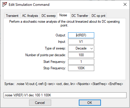
- Output: a point in your circuit where all the individual noise sources will be combined into a single value. “REF” is used here.
- Input: Set “Input” as a noise-free source in the circuit. We use the power supply, V1. LTspice calculates an “equivalent noise input” at the source entered here. We might explore this feature more thoroughly in a future article.
- Type of sweep: Select as with an AC analysis. Decade is used here.
- Number of points per decade: Enter a number to give the desired plotting and analysis resolution; 100 is used here.
- Start Frequency and Stop Frequency: These parameters are similar to the corresponding parameters in an AC analysis; they specify the frequency range of the analysis. However, they also specify the passband to use when LTspice calculates the total noise at the output. There is more on this later. Use 1 and 100K for now.
Click “OK” and place the noise analysis command on the schematic. You can guess the next step. Run the simulation!
Just like in AC analysis, use the probe cursor and click on the REF node. Note that LTspice changes the name of the output plot to “V(onoise)”.
The plot shows a flat line at 9.1 nV/Hz1/2. This is the total of all the individual noise sources added together in an RMS fashion to produce the noise at the output. The vertical axis has units of nV/Hz1/2. This is an obscure unit, and explaining it is beyond the scope of this article. Just know that a noise source described in this way means the noise varies as a function of frequency and is integrated over a frequency range by the square root of the bandwidth. For example, if a noise source is 13 nV/Hz1/2 from 150 Hz to 250 Hz, the total noise in that frequency range is 13 nV/Hz1/2 times the square root of 100, i.e., 13 nV/Hz1/2 × 10 Hz1/2 = 130 nV RMS.
Click on the body of R1. This adds a plot of the noise at the output coming from only R1. It is a flat line at 6.4 nV/Hz1/2.
Simulation 2: Adding a Filter
Next, add a capacitor to filter noise from the power supply. The capacitor also filters noise from R1 and R2. Run the same simulation again. Noise at low frequencies has not changed, but noise is filtered out at higher frequencies. The resistors and capacitor form a low-pass filter.
Put the cursor over C1. No probe! Pure capacitors are considered to be noise-free, and there is nothing to plot. Add resistance to the capacitor (such as leakage resistance), and the probe appears so that you can plot this resistance.
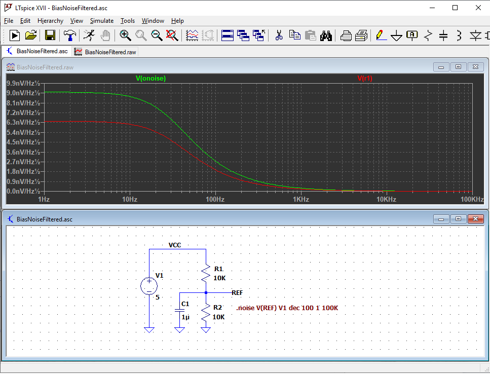
Now we have a great tool to explore tradeoffs and get greater insight into the circuit’s noise performance. For example, R1 and R2 can be made smaller to reduce their thermal noise, but this uses more power, and C1 must be larger in order to keep the same low-pass-filter characteristics.
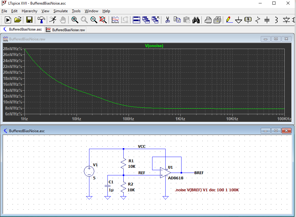
Simulation 3: Adding a Buffer Amplifier
A variation of the bias circuit is to buffer the resistive divider with a voltage follower. We add an op-amp selected for high output current, wide bandwidth, and ability to drive a fairly large capacitive load. This part is in the standard LTspice “Opamps” library. Run the same simulation, but change the simulation output to “BREF”.
Yikes! The lower-frequency noise has gone way up due to 1/ƒ noise from the op-amp, and the higher-frequency noise has returned because the additional noise of the op-amp is not filtered out. Right away we see that the op-amp noise is much greater than the noise from the resistive divider, especially at low frequencies.
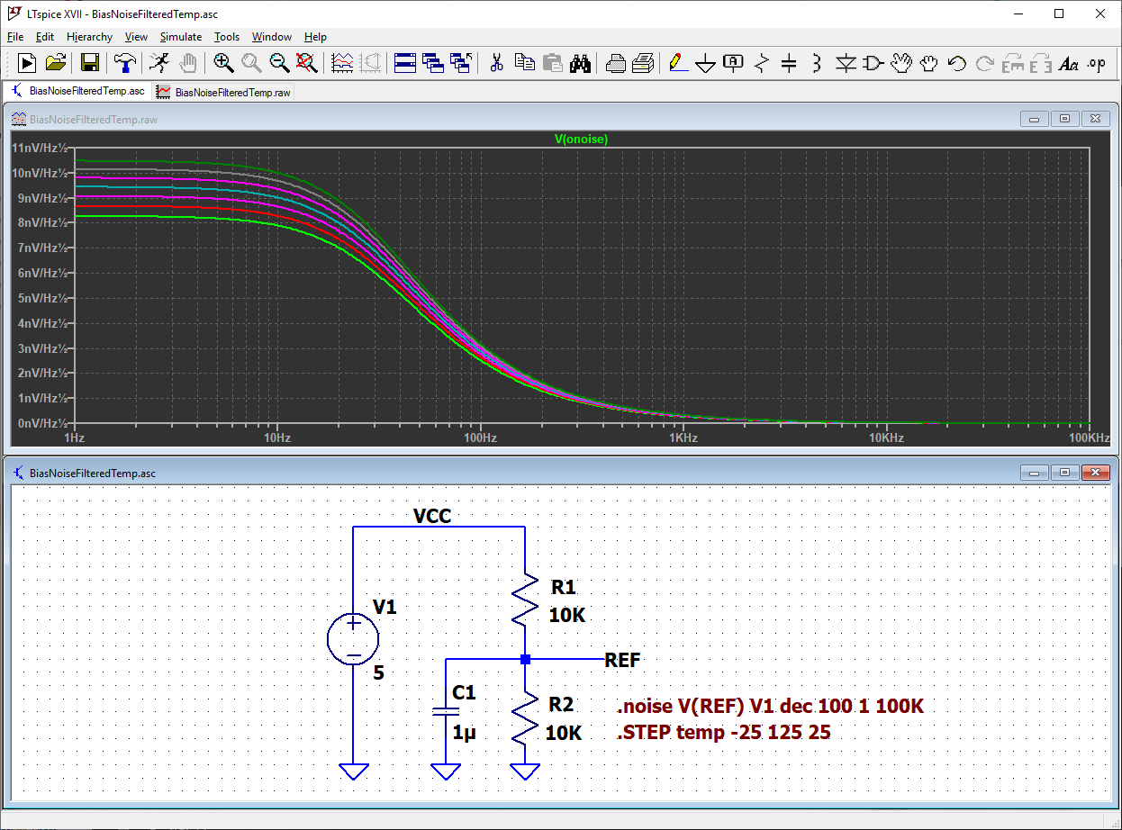
Simulation 4: Temperature
What about temperature? The default in LTspice is 27°C. Modeling noise at different temperatures is done with .STEP or .OPTIONS directives. The “temp” variable is built into LTspice.
The next plot shows the noise over the temperature range -25°C to 125°C in 25°C steps, specified with a .STEP directive. A single temperature can be specified with a .OPTIONS directive. For example, “.OPTIONS temp = 100”.
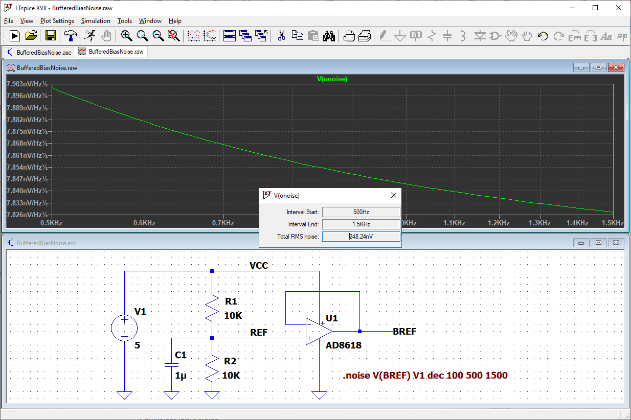
Total Output Noise
At some point, you want to know the total noise as a single voltage. LTspice calculates the total noise within a frequency band by first running the simulation over the frequency band of interest. For example, use 500 Hz to 1500 Hz. Then, plot the output noise. While holding down the CTRL
Some Limitations
- The total noise calculation uses an ideal, squared-off passband. Total noise at the output must be adjusted for real passband shapes.
- Resistors are modeled as ideal thermal noise sources. Real resistors can have additional noise called “excess noise”.
- Op-amp noise modeling in the 1/ƒ region may not be accurate.
Undocumented Bonus Tip
LTspice allows the noise in a resistor to be ignored in the analysis. For example, a large feedback resistor in an op-amp circuit can dominate the noise and make it difficult to see the contribution of the op-amp.
You can turn off the resistor noise by adding the word “noiseless” after the value of the resistor in the schematic. For example, a value of “10Meg” becomes “10Meg noiseless”. In Figure 4, add “noiseless” to the value of R1 and R2 to see the noise from only U1. Low-noise design with LTspice is easy—just use “noiseless” to improve your design!


In the “Total Output Noise” section… You need to hold down the “CTRL” key, to see the total RMS Noise Voltage.
Rather than “the key” —> “Then, plot the output noise. While holding down the key, left click on the V(onoise) label at the top of the plot.”
Hi,
I want to complement that the “input” source can both be voltage source and current source.
And the LTSPICE software will calculate an equivalent input-referred noise density spectrum. If you want to see this, just substitute “V(onoise)” to “inoise”