Noise in Electronics Engineering: Distribution, Noise RMS and Peak-to-Peak Value, and Power Spectral Density

In a previous article, we discussed that the probability density function (PDF) of noise amplitude allows us to extract some precious information such as the mean value and average power of the noise component. While the PDF allows us to estimate the average power of noise, it doesn’t reveal how the noise power is distributed in the frequency domain.

In this article, we’ll first examine an important feature of common noise sources: the relationship between the noise root mean square (RMS) and peak-to-peak value. Then, we’ll see that it’s possible to have an estimate spectrum of the noise sources that are of interest to us.

 

Gaussian or Normal Distribution

In the first part of this article, we took 100,000 samples from an example noise signal and used them to create a histogram of the noise amplitude distribution. Normalizing the histogram gave us an estimate of the noise amplitude PDF. The estimated PDF is shown in Figure 1.

 

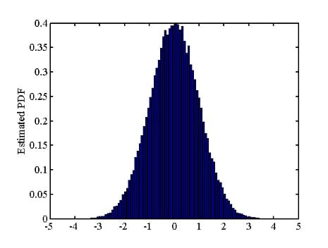
Figure 1

 

The distribution in Figure 1 is actually an estimation of a well-known PDF called the Gaussian or normal distribution which is given by the following equation:

 

\[p_X(x)=\frac{1}{\sigma \sqrt{2\pi}}exp\left ( - \frac{(x-\mu)^2}{2\sigma^2} \right )\]

Equation 1

 

where σ and μ are the standard deviation and mean of the distribution, respectively. We previously discussed that the PDF of the noise amplitude can be used to estimate the mean and variance of the noise signal. If we plug the values from Figure 1 in the mean and variance equations, we’ll obtain a mean and variance of about 0 and 1, respectively. Let’s compare the estimated PDF, which looks like a Gaussian distribution with σ²≈1 and μ≈0, with the exact values for the normal distribution given by Equation 1 (for the same mean and variance values). This is shown in Figure 2. As you can see, the normal distribution with σ=1 and μ=0 very well matches our estimated PDF.

 

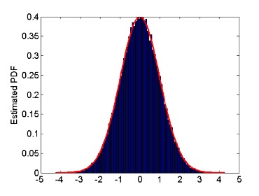
Figure 2

 

Interestingly, many of the common noise sources, such as the noise produced by a resistor, exhibit a Gaussian distribution. 

 

Noise RMS and Peak-Peak Value

Now that we know many noise sources have the amplitude distribution given by Equation 1, can we develop a relationship between the PDF characteristics and the noise peak-to-peak value? Yet a better question: How can we consider a peak-to-peak value for a random signal? Figure 2 suggests that the probability of the noise amplitude being larger than 4 is low; however, this probability is not really zero. 

For a random signal, we can only define a peak-to-peak value. As shown in Figure 3, for a Gaussian distribution with mean value of μ and a standard deviation of σ, about 68.27% of the samples are within one standard deviation of the mean value (μ). Moreover, 95.45% and 99.73% of the noise samples are within 2σ and 3σ of the mean value, respectively.

 

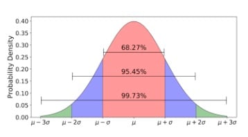
Figure 3. Image courtesy of Towards Data Science

 

Based on the above information, we can assume that the noise peak-to-peak value is equal to six times the distribution’s standard deviation (6σ). In this case, we can expect that about 99.73% of the noise samples are within the range from μ-3σ to μ+3σ. In other words, for about 99.73% of the noise samples, the peak-to-peak value cannot exceed 6σ. Put slightly differently, with a probability of 0.9973, the peak-to-peak value of the noise will be less than 6σ. If we assume that the mean value of the noise is zero, the noise amplitude will be less than 3σ with a probability of 0.9973.

It’s important to note that this is just one way to define the noise peak-to-peak value. Another common definition considers 6.6σ as the noise peak-to-peak value. With this definition, about 99.9% of the samples will give a peak-to-peak value less than 6.6σ. If the mean value is zero, with a probability of 0.999, the noise samples will have an amplitude less than or equal to 3.3σ.

Note that if the mean value of the noise is zero, the standard deviation will be equal to the noise RMS value. When assessing the noise of analog components, we commonly need to convert the peak-to-peak noise to the RMS value and vice versa. To this end, depending on how we define the peak-to-peak value, we can use either of these two formulas: \(6 \times V_{noise, rms}= V_{noise, p-p} \: \: \: or \: \: \:6.6 \times V_{noise, rms}= V_{noise, p-p}\). Please refer to this article for an example of using this information when choosing the appropriate reference voltage IC for an A/D converter.

 

Power Spectral Density

While the PDF allows us to estimate the average power of noise, it doesn’t reveal how this given noise power is distributed in the frequency domain. To better understand why the total average power of a signal does not specify the signal frequency content, consider these two deterministic signals:

 

\[s_1(t)=Asin(2\pi \times 1 \times t)\]

\[s_2(t)=Asin(2\pi \times 10^9 \times t)\]

 

The average power of these two signals is the same and is proportional to \(\frac {A^2}{2}\). However, they have different frequency content. s₁(t) has a frequency component at 1 Hz, whereas s₂(t) has a frequency component at 1 GHz! Similarly, the average power of noise does not determine its frequency content. The PDF shows the distribution of sample amplitudes, but it does not give us any information about how fast the noise samples vary. Just as for a deterministic signal, the faster the noise samples vary in the time domain, the more the signal power will be concentrated at higher frequencies. 

To characterize the frequency content of a noise source, we measure the average power of noise at different frequencies within the bandwidth of interest. For example, to find the noise average power at f₁, we can theoretically apply the noise samples to an ideal bandpass filter with a bandwidth of 1 Hz and center frequency tuned to f₁. This ideal bandpass filter will attenuate all the frequency components outside its 1-Hz bandwidth. The average power measured at the output of the bandpass filter (S_X(f₁)) is an estimate of the average power the noise source can exhibit at f₁. This is illustrated in Figure 4.

 

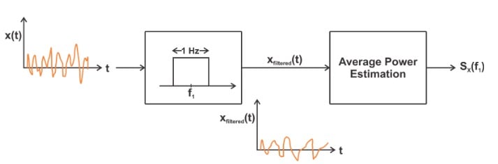
Figure 4

 

We can repeat the above procedure for other frequencies within the bandwidth of interest. This will give us the noise average power versus frequency as shown in Figure 5.

 

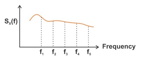
Figure 5

 

These measurements specify the frequency content of the noise, which is usually referred to as the noise power spectral density (PSD). Since we used 1-Hz bandpass filters to measure the average power, the values of the PSD plot will be in V²/Hz. Moreover, manufacturers commonly specify their product noise performance by providing the square root of the PSD. In this case, the unit will be \(V/\sqrt{Hz}\). Noting the provided unit can allow us to recognize whether the noise power or voltage density versus frequency is given.

Additionally, noise is sometimes specified in amps per root Hertz (\(A/\sqrt{Hz}\)). In the next article, we’ll see that the PSD concept is a powerful tool that allows us to examine the effect of a noise source on the output of a system.

 

Conclusion

In this article, we first examined an important feature of common noise sources: the relationship between the noise RMS and peak-to-peak value. We saw that the noise peak-to-peak value is about six times its RMS value. This relationship becomes particularly important when assessing the noise performance of analog components. Then, we looked at the definition of noise PSD which allows us to have an estimate of the noise spectrum.

To see a complete list of my articles, please visit this page.