How to Measure Gas Flow in a Mechanical Ventilator Using a Differential Pressure Sensor

In a previous article in this series, we saw that pressure sensors are key elements of mechanical ventilation. In addition to measuring the airway pressure and the barometric pressure, pressure sensors can also adjust the oxygen concentration of the delivered breath.

In this article, we’ll look at another interesting application of pressure sensing in mechanical ventilation—that is, measuring gas flow using a differential pressure sensor. We will first look at two basic concepts from fluid mechanics: Bernoulli’s equation and the continuity equation. Then, combining these two concepts, we’ll derive an equation that relates the volumetric flow rate to a differential pressure value.    

 

Bernoulli’s Equation

Assume that fluid flows through a pipe with a varying cross-section as shown in Figure 1. The fluid enters the left cross-section and exits the right end of the pipe. 

 

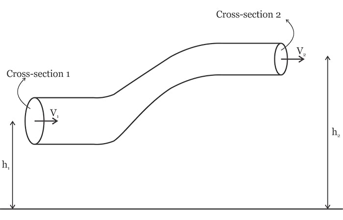
Figure 1. Diagram of a pipe with varying cross-sections.

 

In the above figure, h₁ and h₂ denote the height of the fluid above the earth’s surface at cross-sections 1 and 2, respectively. With a pipe diameter much smaller than the pipe height, we can assume that all of the fluid particles at a given cross-section are almost at the same height. Applying the law of conservation of energy to the fluid particles at cross-sections 1 and 2, we can derive the following equation:

 

\[P_1+\frac{1}{2}V_1^2+\rho gh_1=P_2+\frac{1}{2}V_2^2+\rho gh_2\]

 

where P is the fluid pressure, ρ is its density, V denotes the fluid velocity, and g is the acceleration due to gravity. The variables with subscripts ₁ and ₂ correspond to the fluid parameters at cross-sections 1 and 2, respectively.

The above equation is often referred to as Bernoulli’s equation. This is not a new law of physics and is simply a consequence of the law of conservation of energy: the energy at pipe input should be equal to the energy at the output. The pressure term of Bernoulli’s equation is related to the work done on the fluid by the fluid particles behind a given cross-section.

The second term of Bernoulli's equation denotes the fluid kinetic energy and the third term corresponds to its potential energy. For the proof of Bernoulli’s equation, you can refer to this video on Bernoulli's equation derivation. Note that Bernoulli’s equation is valid for incompressible, nonviscous fluids that flow in a non-turbulent, steady-state manner.

For the special case of \(h_1 \approx h_2 \), Bernoulli’s equation simplifies to:

 

\[P_1+\frac{1}{2}\rho V_1^2=P_2+\frac{1}{2}\rho V_2^2\]

Equation 1

 

Equation of Continuity

According to the principle of mass conservation, mass can be neither created nor destroyed. This principle from classical mechanics along with some assumptions about the fluid flow can help us relate the cross-sectional area that the fluid goes through (A) to the fluid velocity (V). Consider the steady flow of a fluid through a pipe with a varying cross-section as shown in Figure 2. 

 

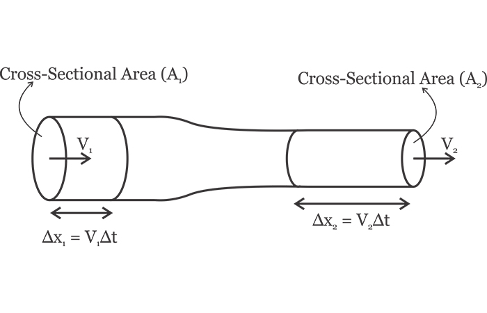
Figure 2. A steady flow through a pipe with varying cross-sections.

 

With a steady flow, the velocity, density, and pressure of the fluid at a given point do not change with time. 

Assume that the fluid enters the left end of the pipe at a velocity of \(V_1\). The fluid particles that go past the cross-sectional area \(A_1\) will travel by \(\Delta x_1 \) after a small time interval of \(\Delta t \).

The distance traveled can be expressed in terms of velocity as \(\Delta x_1 = V_1 \Delta t \). That said, the volume of the fluid that enters the pipe in a time interval of \(\Delta t \) is \(A_1 V_1 \Delta t \). Multiplying this value by the fluid density gives us the mass that enters the pipe as \(\rho A_1 V_1 \Delta t\). Similarly, we can calculate the mass that exits the right end of the pipe as \(\rho A_2 V_2 \Delta t\).

According to the principle of mass conservation, the mass that enters the pipe should be equal to the mass that exits it. Hence, we have

 

\[\rho A_1 V_1 \Delta t = \rho A_2 V_2 \Delta t\]

 

which simplifies to:

 

\[A_1 V_1=A_2 V_2\]

Equation 2

 

This equation is the continuity equation for one-dimensional flow. It states that the product of the cross-sectional area and the fluid velocity at that cross-section is constant.

The above derivation is based on a few assumptions about the fluid flow. For example, we assume that the fluid velocity and density at a given point do not change with time (the flow is steady). Besides, the fluid density at the left end of the pipe is equal to the fluid density at the right end. In other words, the fluid is incompressible. 

 

Calculating Flow Rate from a Pressure Differential

Using Bernoulli’s equation along with the continuity equation, we can find the volume of the fluid that flows per second. In fluid dynamics, the parameter that specifies the number of cubic meters of fluid that flows per second (expressed in terms of \(\frac {m^3}{s}\)) is called the volumetric flow rate. Based on this definition, the volumetric flow rate, denoted by Q, is given by:

 

\[Q=\frac{Volume}{time}\]

 

The volume of the fluid that goes past a cross-section of pipe in a given time interval (\(\Delta t \)) can be expressed as the product of the pipe cross-sectional area (A) times the distance the fluid travels (\(\Delta x \)). 

 

\[Q=\frac{Volume}{time} =\frac{A\times \Delta x}{\Delta t} =AV\]

 

where \(\frac{\Delta x}{\Delta t}\) is substituted by the fluid velocity V. Hence, we can calculate the volumetric flow rate of a fluid by simply measuring the fluid velocity. The velocity measurement can be achieved by applying the concepts discussed above to a pipe with a varying cross-section as shown in Figure 3. 

 

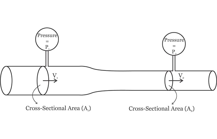
Figure 3. Depiction of how to find the velocity measurement to a pipe with different cross-sections.

 

Note the two ports that are connected to pressure sensors to measure the pressure difference along the pipe. 

Based on Equation 1, we have

 

\[\Delta P=P_1-P_2=\frac{1}{2}\rho \left ( V_2^2-V_1^2 \right )\]

 

Substituting Equation 2 into the above equation gives us:

 

\[\Delta P=\frac{1}{2}\rho V_2^2 \left (1-\left (\frac{A_2}{A_1} \right )^2 \right )\]

 

This equation relates the fluid velocity (V2) to the differential pressure and the pipe dimensions. Now, we can calculate the volumetric flow rate (Q) of the fluid as:

 

\[Q=A_1V_1=A_2V_2=A_2\sqrt{\frac{\Delta P \times 2}{\rho \left (1-\left ( \frac{A_2}{A_1} \right )^2 \right )}}\]

Equation 3

 

Measuring the Volumetric Flow Rate of a Gas

Both Bernoulli’s equation and the continuity equation are derived based on the assumption that the fluid is incompressible. In general, gases are compressible and we cannot use the above method to measure the flow rate of a gas.

However, when the velocity of a gas is sufficiently below the speed of sound, the variation of the gas density becomes negligible and we can assume that it is incompressible. Besides, for a gas to be treated as incompressible, the temperature should not change significantly along its flow path. Fortunately, there are applications, such as gas flow in a mechanical ventilator, that satisfy these conditions. 

 

Measuring Gas Flow in a Mechanical Ventilator

Some ventilators and spirometers use the method described in this article to measure the air that moves in and out of a patient’s lungs. To experiment with the concepts discussed here, you can 3D print a tube similar to the one shown in Figure 3, though you might have to do several experiments before finding the appropriate dimensions for the tube. For a given tube, equation 3 can be rewritten as

 

\[Q=A_2\sqrt{\frac{\Delta P \times 2}{\rho \left (1-\left ( \frac{A_2}{A_1} \right )^2 \right )}}=k_{system}\sqrt{\Delta P}\]

 

where \(k_{system} \) is a constant value that relates the differential pressure to the gas flow. If you have access to a machine that blows a specific quantity of air within a known period of time, you can do some experiments to measure the system constant rather than calculating it. 

An alternative solution is using a commercially-available pneumotach. As shown in Figure 4, a pneumotach inserts a light screen in the airflow to create a known pressure drop that is directly proportional to the air velocity. 

 

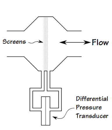
Figure 4.  Light screen inserted in the airflow to create a pressure drop proportional to the air velocity. Image used courtesy of Richard Johnston [CC BY-NC 4.0]

 

You can find more information about this method Richard Johnston's article on the basics of pneumotach flow measurement. 

 

Conclusion

In this article, we introduced a method for measuring gas flow in mechanical ventilation. This method is based on two basic concepts from fluid mechanics: Bernoulli’s equation and the continuity equation. Combining these two concepts gives us an equation that relates gas flow to the pressure difference along the pipe.

In addition to the technique discussed here, there are several other methods for measuring gas flow. Some of these techniques are more linear than others but none of them are perfectly linear. A flow sensor based on a commercially available pneumotach can be one of the most linear methods of measuring gas flow rate. 

To see a complete list of my articles, please visit this page.